Numerical Indications of Localization

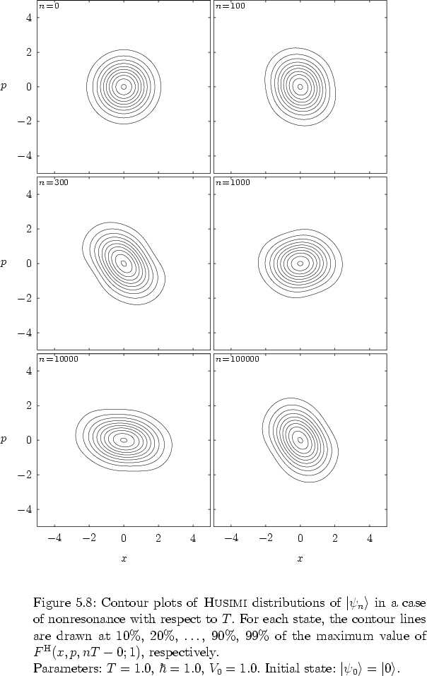
In chapter 4 I have shown how the quantum manifestations of classical stochastic webs develop under iteration of the quantum map of the kicked harmonic oscillator. Now I turn to the complementary case of nonresonance, in which classically no stochastic web is present and typically the system is characterized by diffusive classical dynamics if $V_0$ is sufficiently large.

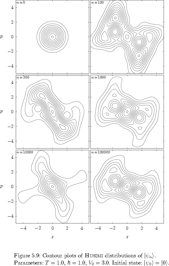
Figure 5.9

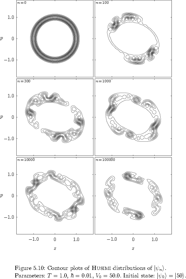
shows the time evolution of an initial coherent state, centered at $(0,0)^t$, under the dynamics of the quantum map (2.37) for the nonresonant $T=1.0$. This figure is to be compared with figure 1.4 showing a phase portrait of the corresponding classical dynamics. In agreement with the classical case there is no spreading of the quantum wave packet; it is just slightly deformed under the dynamics of the quantum map. This observation is not too surprising, as the given initial state $\left \vert 0 \right >$ is concentrated in the phase space region that is surrounded by the yet unbroken outer invariant line visible in figure 1.4.

This changes in figure 5.10,

which shows the same as figure 5.9, but for a larger value of $V_0$: $V_0=3.0$. Classically, for this $V_0$ the last remaining invariant line has already broken up and given way for global diffusive dynamics of any ensemble of initial conditions. But the quantum dynamics in figure 5.10 shows no sign of any corresponding spreading of the initial wave packet. It is distorted slightly more than in the previous figure, due to the larger $V_0$, but obviously it does not flow apart. Even after $10^5$ iterations of the quantum map the wave packet is well localized. There is no indication of further spreading beyond what is already seen, for example, after 100 kicks.

Figure 5.11

supports this observation. The figure displays the time evolution of the quantum states for a smaller value of $\hbar$: $\hbar =0.01$; accordingly, $\left\vert \psi_0 \right>=\left\vert 50 \right>$ has been chosen for the initial state. -- Cf. equation (4.4) in subsection 4.1.1 for an explanation of this choice for the initial state. -- Again obviously localized quantum dynamics is found, even though for this figure the kick strength has been chosen very large, $V_0=50.0$, such that in classical mechanics strongly diffusive dynamics would have been expected.

Some further remarks on the choice of the initial state: While the preceding figures for $\hbar =1.0$ had $\left\vert \psi_0 \right>=\left\vert 0 \right>$, in figure 5.11, for the lower value of $\hbar$, I have $\left\vert \psi_0 \right>=\left\vert 50 \right>$. As discussed earlier, this choice has the advantage that energies of the respective initial states are the same, roughly, for all three figures: $\hbar/2\vert _{\hbar=1.0}=0.5 \approx \hbar(50+1/2)\big\vert _{\hbar=0.01}=0.505$. In addition, in this way all three initial states cover approximately the same area in phase space (near the classical path of the harmonic oscillator with $E=0.5$.), thus facilitating the comparison of the corresponding phase space distributions. What is more, the alternative possibility of choosing $\left\vert \psi_0 \right>=\left\vert 0 \right>$ for all values of $\hbar$ would have the disadvantage of already starting with states that are more localized for smaller values of $\hbar$.

The numerical evidence collected by iterating the quantum map for many different combinations of parameters and initial states -- in addition to the figures shown here, a small selection of these simulations is documented in section C.4 of the appendix -- indicates that regarding localization the dynamics is ``robust'' with respect to the initial state: having iterated just long enough, for a given parameter combination always the same type of quantum dynamics evolves, regardless of the exact choice of $\left\vert \psi_0 \right>$ -- as long as $\left\vert \psi_0 \right>$ is concentrated in a phase space region that is characterized by localized dynamics. (But also take into account the considerations in subsection 5.2.2 concerning the choice of the initial position of $\left\vert \psi_0 \right>$ in quantum phase space.) In this sense the notion of arbitrariness that entered the discussion via the ad hoc choice of initial conditions is rendered irrelevant.

The above observations on the lack of quantum phase space diffusion are fairly convincing, as the quantum map has been iterated a very large number of times, up to and beyond $n=10^5$, and the available numerical indications show that the computations are not too erroneous: typically, the error of the norm of the numerically computed states does not exceed $10^{-10}$, and often it is even much smaller. Observations of the same kind can be made for ``any'' other combination of parameters, as long as $T$ takes a nonresonant value. The situation becomes completely different in the resonance case, of course, as discussed in chapter 4. Some more examples of HUSIMI contour plots demonstrating localization in quantum phase space can be found in section C.4 of the appendix.

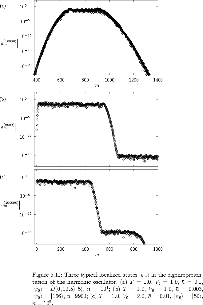
Another manifestation of this localization is obtained by plotting the expansion coefficients $a_m^{(n)}$ -- cf. the expansion (2.40) -- of wave packets that have been generated by iterating the quantum map (2.37) $n$ times, with $n$ sufficiently large. Figure 5.12

shows typical states in this eigenrepresentation $\{\left\vert m \right>\}$ of the harmonic oscillator. The exponential decay of the absolute values of the expansion coefficients to the right -- and in figures 5.12a and 5.12b to varying degree to the left as well -- is clearly visible. The nonexponential parts on the right hand sides of figures 5.12b and 5.12c are noise-floors, due to the unavoidable numerical errors in the computation; they do not interfere with the above interpretation of these graphs.

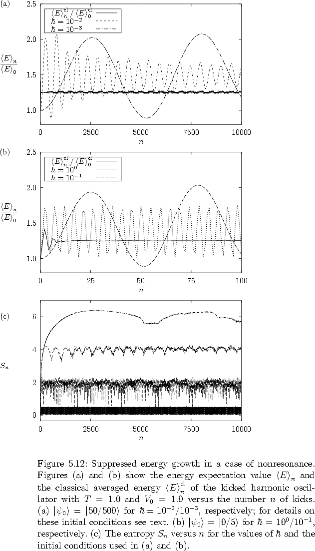
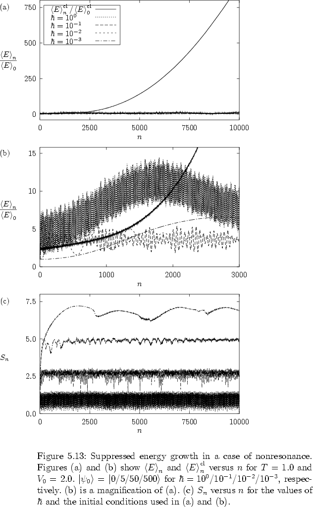
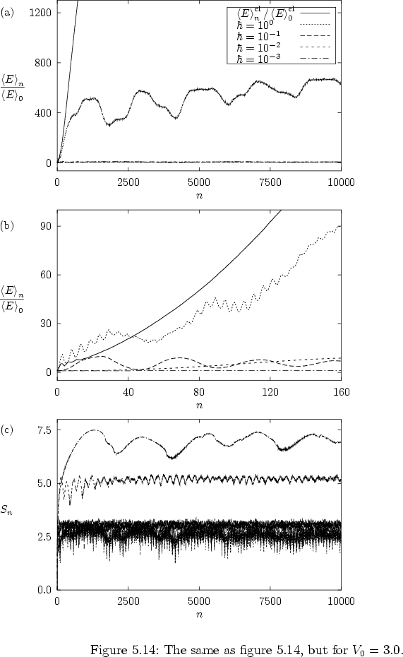
In order to get a less qualitative picture of the situation it is useful -- although less intuitive than looking at quantum phase space pictures -- to consider the behaviour of the energy expectation value (4.5) of the system as a function of time. Figures 5.13a,b/5.14a,b/5.15a,b,

(corresponding, for $\hbar =1.0$, to figures 5.9, C.41 and 5.10, for example) show the time evolution of quantum energy expectation values $\left< E \right>_n$ of the kicked harmonic oscillator for $V_0=1.0/2.0/3.0$ and $T=1.0$, i.e. in cases of classical nonresonance, for several values of $\hbar$. For the computation of the corresponding ensemble averaged classical energy $\left< E \right>_n^{\rm cl}$ (cf. equation (1.74)) an ensemble of initial values has been used that is described by the same Gaussian in phase space as the HUSIMI distribution for the coherent state  $\left \vert 0 \right >$.

In line with the above remarks concerning the case of $V_0=1.0$, figure 5.13 shows no unexpected deviation of the quantum energy expectation values from the classical energy averages (disregarding the typical quantum mechanical oscillations of $\left< E \right>_n$ around the classical value of $\left< E \right>_n^{\rm cl}$); in both the quantum and the classical cases the dynamics is localized and therefore the energy is bounded. As indicated by the previous figures, the situation is different for larger values of $V_0$, as displayed in figures 5.14 and 5.15: in contrast to the classical energies which grow without upper bound, the quantum curves (for all values of $\hbar$ considered) obviously are characterized by bounded energy growth. This is a clear indication to quantum suppressed energy growth, i.e. quantum localization, similar to the quantum localization demonstrated in figure 5.4 with respect to the quantum kicked rotor.

Figures 5.13c/5.14c/5.15c show another manifestation of quantum localization: in these figures the entropy (4.9) of the iterated quantum states is plotted, also exhibiting saturation after a limited number of iterations. The entropy is a good means for demonstrating localization, as by definition it measures the degree to which a state spreads within the HILBERT space of kicked harmonic oscillator states, and thereby in phase space -- cf. subsection 4.1.2.

Using a different kick function (making the system much more tractable numerically but not allowing for stochastic webs to develop), a similarly slowed down energy growth in a related version of the quantum kicked harmonic oscillator has been observed numerically in [SHM00], but the authors could not provide an analytical explanation for their observation.