In subsection 1.2.4 I have discussed the diffusive energy growth in the channels of classical stochastic webs, i.e. in the cases of resonance given by equation (1.33). In the present subsection I study the quantum energy growth in these cases leading to the emergence of quantum stochastic webs, as shown in subsection 4.1.1 and in sections C.1 and C.2 of the appendix.
display the quantum energy expectation value![$V_0{ {\protect\begin{array}{c}
>\protect\\ [-0.3cm]\sim
\protect\end{array}} }10.0$](img707.png) can lead to
a very fast spreading of the states and thus may necessitate to
stop the algorithm after only a short period of time.
For comparison, results for
can lead to
a very fast spreading of the states and thus may necessitate to
stop the algorithm after only a short period of time.
For comparison, results for
Within the accuracy of the computation, the figures indicate that
for generic values of ![]() -- here: for
-- here: for ![]() ; nongenericity of
; nongenericity of ![]() in the present
context is defined in equations (4.7) below --
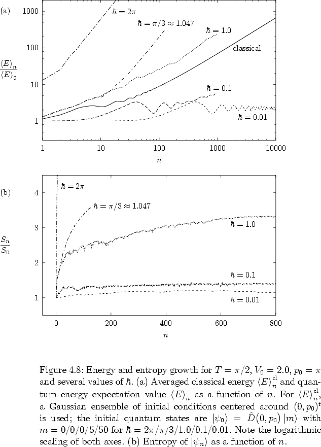
the quantum energy grows in the same way as the classical energy average
does: in the doubly logarithmic plots, the slopes of the respective
graphs indicate an asymptotically linear dependence on time,
in the present
context is defined in equations (4.7) below --
the quantum energy grows in the same way as the classical energy average
does: in the doubly logarithmic plots, the slopes of the respective
graphs indicate an asymptotically linear dependence on time,
Many more results of this kind, for other values of generic ![]() and
and
![]() , have been obtained numerically, but are not shown here.
Similarly, numerical results with respect to the third
nontrivial
type of resonance, given by
, have been obtained numerically, but are not shown here.
Similarly, numerical results with respect to the third
nontrivial
type of resonance, given by ![]() , are not shown here either, but
have been obtained in large numbers; they lead to
similar observations as described above.
Summarizing I have the result that, generically, in quantum mechanics
diffusive energy growth within stochastic webs is obtained, just as
in the classical case.
, are not shown here either, but
have been obtained in large numbers; they lead to
similar observations as described above.
Summarizing I have the result that, generically, in quantum mechanics
diffusive energy growth within stochastic webs is obtained, just as
in the classical case.
The figures also show results for some nongeneric values of
![]() . In the present context,
. In the present context, ![]() is called nongeneric if there is
an integer
is called nongeneric if there is
an integer ![]() such that
such that
This definition of nongenericity of ![]() is based on equations
(4.44) and (4.49) below, which are obtained
in a natural way
in subsection 4.2.2
when analytically discussing
dynamical consequences of the symmetries of quantum stochastic webs.
The cases of nongeneric
is based on equations
(4.44) and (4.49) below, which are obtained
in a natural way
in subsection 4.2.2
when analytically discussing
dynamical consequences of the symmetries of quantum stochastic webs.
The cases of nongeneric ![]() as given by equations
(4.7) are examples of quantum resonances;
this is explained in subsection 4.2.2 as well.
as given by equations
(4.7) are examples of quantum resonances;
this is explained in subsection 4.2.2 as well.
With more than convincing numerical accuracy, the figures
-- with ![]() and
and ![]() in figure
4.8, and
in figure
4.8, and
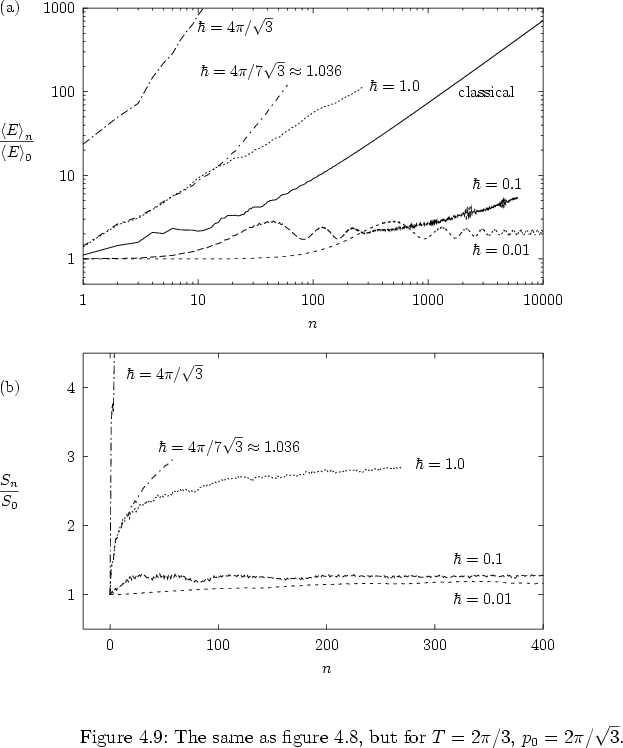
![]() and
and ![]() in figure
4.9 --
indicate that
these
nongeneric
values of
in figure
4.9 --
indicate that
these
nongeneric
values of ![]() asymptotically lead to faster, namely quadratic,
energy growth,
asymptotically lead to faster, namely quadratic,
energy growth,
![$n{ {\protect\begin{array}{c}
<\protect\\ [-0.3cm]\sim
\protect\end{array}} }10$](img716.png) the curves for
the curves for
Both energy growth rate results,
diffusive (4.6) and
ballistic (4.8),
are given a theoretical explanation in
section 4.2.
Note that, irrespective of the (non-) genericity of the value of ![]() ,
for a given resonant
,
for a given resonant ![]() always the same symmetric phase space patterns
are obtained. In other words, depending on the value of
always the same symmetric phase space patterns
are obtained. In other words, depending on the value of ![]() , the same
quantum stochastic web may be subject to diffusive or ballistic energy
growth of the quantum state moving within the web.
, the same
quantum stochastic web may be subject to diffusive or ballistic energy
growth of the quantum state moving within the web.
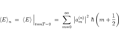
Considering the diffusive energy growth of the quantum states
![]() is one way of discussing the spreading of the states
in the phase plane with time.
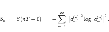
Another way is to discuss their VON NEUMANN entropy
is one way of discussing the spreading of the states
in the phase plane with time.
Another way is to discuss their VON NEUMANN entropy