Diffusive Energy Growth in the Channels

The time evolution of the stochastic web shown in figure 1.7 allows the conclusion that with a growing number of iterations of the web map an increasingly large region of phase space is covered by orbit points. This observation can be cast into a more exact form by considering the energy

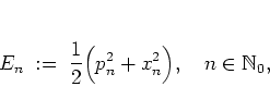$$E_n \; := \; \frac{1}{2}\Big( p_n^2 + x_n^2 \Big), \quad n\in\mathbb{N}_0,$$ (1.46)

for a particle moving within the stochastic web. Obviously, $E_n$ is the well-defined energy only between the kicks, namely between the $(n-1)$-st and the $n$-th kick. $E_n$ grows quadratically with the distance of the particle from the origin of the phase plane.

Figure 1.16

Figure 1.16: The energy $E_n$ of the kicked harmonic oscillator for $q=4$ ($T=\pi /2$) versus the number $n$ of kicks. (a) $V_0=1.0$; (b) $V_0=2.0$. The initial values are $(0,p_0)^t$ with the values of $p_0$ given in the insets.

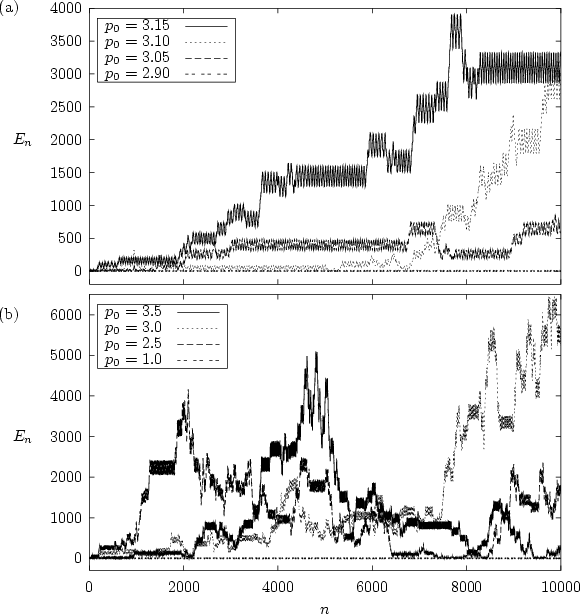shows how, for $q=4$, the energy develops as a function of time for some typical orbits and for two different values of $V_0$. Two entirely different types of motion can be distinguished: first, if the initial condition $(x_0,p_0)^t$ of the orbit is chosen from one of the regular regions where invariant lines persist, then $E_n$ remains bounded as the orbit revolves on its corresponding invariant line. The orbits with $p_0=2.9$ in figure 1.16a and $p_0=1.0$ in figure 1.16b are of this type, giving rise to the nearly horizontal lines at $E_n\approx 0$. Second, for initial conditions within the channels of the web, unbounded motion is possible and dominates the dynamics. The other orbits in figure 1.16 correspond to initial conditions of this class. This type of motion manifests itself by sharp increases and declines in the energy. Between the times of rapidly changing energy there are time intervals for which the energy remains roughly constant. The length of these time intervals varies and typically decreases with increasing values of $V_0$.

For orbits of the second type, on the average the energy grows with time; this is the most prominent feature of the dynamics in the channels of the web. For computational convenience this time average can be replaced by an ensemble average. Rather than considering a very long orbit for a single initial condition I generate a family of orbits, corresponding to a Gaussian distribution of initial values, and compute the accordingly averaged energy at time $nT-0$,
denoted by $\left< E \right>_n^{\rm cl}$.^1.10Using an ensemble average also allows for a more straightforward comparison with the quantum dynamics of the system, since in quantum mechanics HEISENBERG's uncertainty relation rules out the possibility of considering $\delta$-shaped initial distributions (corresponding to single classical initial values) in phase space.

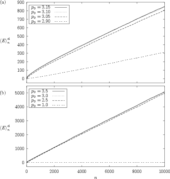
In figure 1.17

Figure 1.17: The averaged energy $\left< E \right>_n^{\rm cl}$ of the kicked harmonic oscillator for $q=4$ ($T=\pi /2$) versus the number $n$ of kicks. (a) $V_0=1.0$; (b) $V_0=2.0$. For each graph $10^4$ initial values are used which are distributed according to a Gaussian with half width 0.1, centered around the same initial values as in figure 1.16.

I employ Gaussian distributions of initial conditions which are centred around the initial conditions of the preceding figure. The Gaussians used here are of half width 0.1, both in $x$- and $p$-direction. From these curves it is quite clear that the gross oscillations seen in figure 1.16 cancel as a result of the averaging over many orbits. Initial distributions centred in regular regions of phase space yield a slower increase of the energy at first, but due to the tails of the Gaussian distributions even in these cases the averaged energy is not bounded any more.

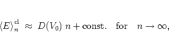
After averaging it becomes obvious that -- apart from a brief
( $n {\protect\begin{array}{c} <\protect\\ [-0.3cm]\sim \protect\end{array}} 1000$) transient stage of subdiffusive motion -- the growth of the energy is characterized by normal or EINSTEIN diffusion [Ein06], i.e. the averaged energy grows as a

linear function of time,

$$% \Erwart{E_n} \approx D n + \mbox{const.} \left< E \right>... ...(V_0) \; n + \mbox{const.} \quad \mbox{for} \quad n\to\infty,$$ (1.47)

with a diffusion coefficient $D(V_0)$. As indicated by the above figures, $D(V_0)$ should be expected to be a function of the amplitude $V_0$ of the kicks, but independent of $n$.

For larger values of $V_0$ a formula for $D(V_0)$ can be derived analytically, which holds (with deviations which are discussed below) for all web maps with $q\in\tilde{{\mathcal Q}}$. From equation (1.21) it follows that for a single orbit the energy change inflicted by the $n$-th kick is determined by

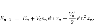$$% E_{n+1} = E_n + V_0p_n\sin x_n + \frac{1}{2}V_0^2\sin^2 x... ...n+1} \; = \; E_n + V_0p_n\sin x_n + \frac{V_0^2}{2}\sin^2 x_n.$$ (1.48)

Averaging over $x_n$ and $p_n$ then gives

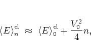$$% \Erwart{E_n} \approx\; \Erwart{E_0} + \frac{1}{4}V_0^2 n,... ...\; \approx \; \left< E \right>_0^{\rm cl} + \frac{V_0^2}{4} n,$$ (1.49)

such that I have for the diffusion coefficient:

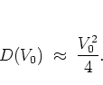$$% D(V_0) \approx \frac{1}{4}V_0^2. D(V_0) \; \approx \; \frac{V_0^2}{4}.$$ (1.50)

This derivation, which is largely analogous to the random phase approximation for the kicked rotor [Chi79,CCIF79] (see also subsection 5.1.1), relies on the straightforward averaging over $x_n$ and $p_n$. Roughly, it can be taken to be justified if unbounded and unhindered motion into all directions of the phase plane is possible, i.e. if $q\in\tilde{{\mathcal Q}}$, and if, in addition, the channels are wide enough, i.e. if $V_0$ is large enough. For aperiodic webs, on the other hand, the dynamics is subdiffusive, because the nonperiodicity implies that in general the channels of the webs are not wide enough everywhere for unrestricted diffusion through all the channels (cf. [Hip94]).

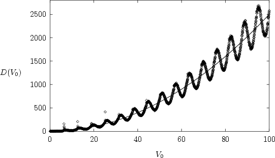
The quality of the approximation leading to equation (1.78) is checked in figure 1.18 for the case of $q=4$.

Figure 1.18: Diffusion coefficients for $q=4$ ($T=\pi /2$). The $\diamond$ indicate least squares approximations of $D(V_0)$ which are determined numerically, based on ensembles consisting of $5\!\cdot\!10^4$ points which are iterated $10^4$ times; the continuous line is the graph of the function (1.78).

For several values of $V_0$ I have calculated $\left< E \right>_n^{\rm cl}$ and obtained $D(V_0)$ using a least squares fit;^1.11these values of the diffusion coefficient are compared with the graph of formula (1.78). By and large, agreement of the two can be observed. But it is also a striking feature of figure 1.18 that an additional oscillation of the diffusion coefficient is found to be superimposed to the expected parabola. Following [KM90] such oscillations of the diffusion coefficient can be attributed to autocorrelations of the orbits, due to small islands of stability in the channels of the web, while strictly speaking the (``quasilinear'') result (1.78) holds for Markovian dynamics only [CM81,Rei98]. For a more detailed analysis of the parameter dependence of the diffusion coefficient for the kicked harmonic oscillator see [DH95,DH97].

Footnotes

....^1.10

The superscript $^{\rm cl}$ is used to distinguish the classical ensemble average $\left< \cdot \right>^{\rm cl}$ from the quantum expectation value $\left< \cdot \right>$.

... fit;^1.11

More sophisticated methods for determining the speed of diffusion can be found in the literature; see for example [Hip94] and references therein.