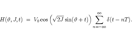
The iteration of the web map (1.24) for ![]() (
(![]() ) typically yields
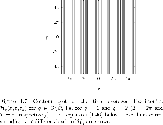
phase portraits like those shown in figure 1.7.
) typically yields
phase portraits like those shown in figure 1.7.
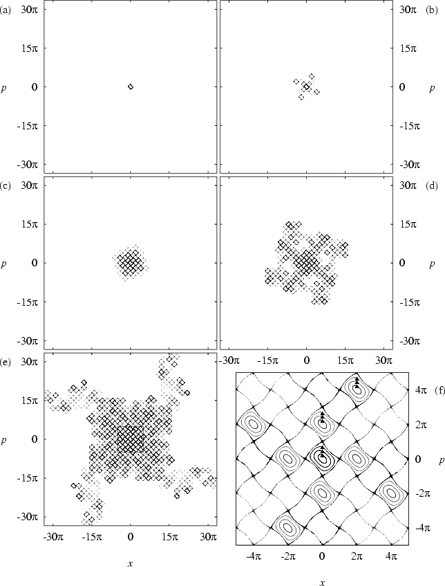 |
Figure 1.8, where phase portraits of the web map for several
values of the
kick amplitude
![]() are shown, allows the conclusion
that the overall structure of the web is the same, regardless of the
value of
are shown, allows the conclusion
that the overall structure of the web is the same, regardless of the
value of ![]() -- the main consequence of increasing the value of
-- the main consequence of increasing the value of ![]() being a broadening of the channels of the web.
being a broadening of the channels of the web.
![\begin{figure}% % % \rule[-0.1cm]{0.0cm}{0.0cm}
\par
\hspace*{-1.5cm}
% \psfig...
...\psfig{file=websq4.eps}
\vspace*{-1.0cm}
% \vspace*{-0.5cm}
\par\end{figure}](img167.png) |
The stochastic webs for ![]() shown in figure 1.8 are
(approximately)
characterized by translational symmetry in two linearly
independent directions (e.g. given by
shown in figure 1.8 are
(approximately)
characterized by translational symmetry in two linearly
independent directions (e.g. given by ![]() and
and ![]() ) and
by two rotational symmetries with respect to
2-fold and 4-fold rotation axes,
in addition to several (glide) reflection symmetries.
More can be said about the symmetries of the skeleton of this web
-- see below.
) and
by two rotational symmetries with respect to
2-fold and 4-fold rotation axes,
in addition to several (glide) reflection symmetries.
More can be said about the symmetries of the skeleton of this web
-- see below.
I now proceed to the explanation of these characteristics of the web
dynamics that
-- for the resonant values ![]() with
with
![]() --
manifest themselves
in figures
1.3a,
1.7 and 1.8.
--
manifest themselves
in figures
1.3a,
1.7 and 1.8.
The overall structure of the web, its skeleton, can be explained by splitting the Hamiltonian (1.17) into two parts, such that the first gives an analytical description of the skeleton and the second can be treated as a perturbation to the first.
In a preliminary step the Hamiltonian (1.17) is submitted to a pair
of successive canonical transformations, the first replacing the original
coordinates ![]() with polar coordinates (which are identical to action-angle variables
of the unperturbed harmonic oscillator except for a sign in
the angle),
while the second switches to a rotating
frame of reference with coordinates
with polar coordinates (which are identical to action-angle variables
of the unperturbed harmonic oscillator except for a sign in
the angle),
while the second switches to a rotating
frame of reference with coordinates ![]() . The combination of both
transformations can be described by the
time-dependent
generating function
. The combination of both
transformations can be described by the
time-dependent
generating function
which is of GOLDSTEIN's ![]() -type [Gol80].
The old and new variables are related via
-type [Gol80].
The old and new variables are related via
![\begin{subequations}
\begin{eqnarray}
J & = & \frac{1}{2}\left(x^2+p^2\right) \\ [0.3cm]
\tan(\vartheta+t) & = & \frac{x}{p},
\end{eqnarray}\end{subequations}](img174.png)
and the new Hamiltonian is obtained as
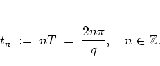
Setting ![]() with
with
![]() ,
,
![]() ,
and using the resonance condition (1.23) I
have
,
and using the resonance condition (1.23) I
have
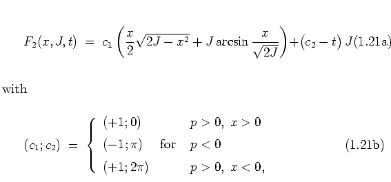
| (1.21) |
 |
(1.22) |
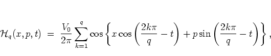
For the present purpose I need
![]() expressed in terms of the
original phase space variables
expressed in terms of the
original phase space variables ![]() . Substitution of the
transformation (1.35) into
the Hamiltonian
(1.39b) yields
. Substitution of the
transformation (1.35) into
the Hamiltonian
(1.39b) yields
 |
(1.22) |
 |
(1.23) |
 |
(1.24) |
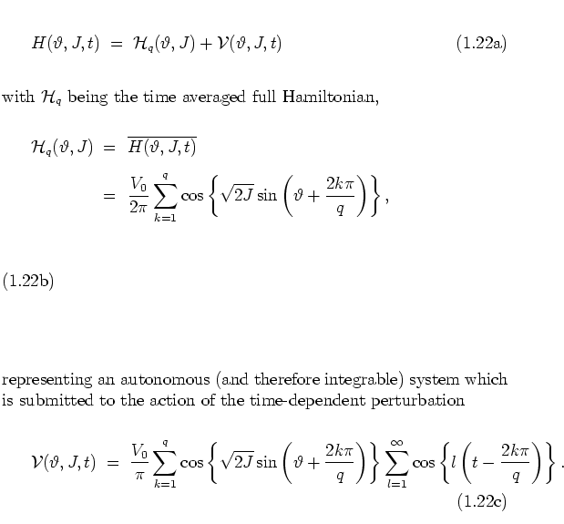
In subsection 1.2.3
I demonstrate that ![]() can indeed be
treated as a perturbation to
can indeed be
treated as a perturbation to
![]() . This means that for
. This means that for ![]() the dynamics of the web map is confined to
the neighbourhood of
surfaces
-- i.e. lines in the
the dynamics of the web map is confined to
the neighbourhood of
surfaces
-- i.e. lines in the ![]() -plane --
of constant
-plane --
of constant
![]() .
For each sufficiently small
.
For each sufficiently small ![]() the skeleton of the web
is
then
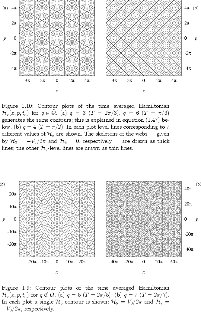
given by some specific contour lines of the time averaged Hamiltonian
(1.43). The term ``specific'' is important here: the
the skeleton of the web
is
then
given by some specific contour lines of the time averaged Hamiltonian
(1.43). The term ``specific'' is important here: the
![]() -level
has to be chosen in such a way that the
corresponding contour lines form an infinitely extended structure, in
fact the skeleton of the stochastic web. The other levels are important,
too; they approximate the bounded quasiperiodic motion in the meshes of the
web and accordingly have the topological structure of circles in the
phase plane.
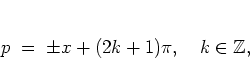
Figures 1.9-1.11
show contour plots for some of the more important
-level
has to be chosen in such a way that the
corresponding contour lines form an infinitely extended structure, in
fact the skeleton of the stochastic web. The other levels are important,
too; they approximate the bounded quasiperiodic motion in the meshes of the
web and accordingly have the topological structure of circles in the
phase plane.
Figures 1.9-1.11
show contour plots for some of the more important
![]() .
.
The case ![]() (
(![]() ) may serve to exemplify the above statements. For this
value of
) may serve to exemplify the above statements. For this
value of ![]() the time averaged Hamiltonian
the time averaged Hamiltonian
Figure 1.10b
is to be compared with the
phase portraits in figures 1.7 and 1.8 that have been
generated by
iteration of ![]() . Going backwards from figure 1.8f to
1.8a,
. Going backwards from figure 1.8f to
1.8a, ![]() tends to zero, and accordingly the stochastic
webs more and more approach the rectangular grid of figure
1.10b.
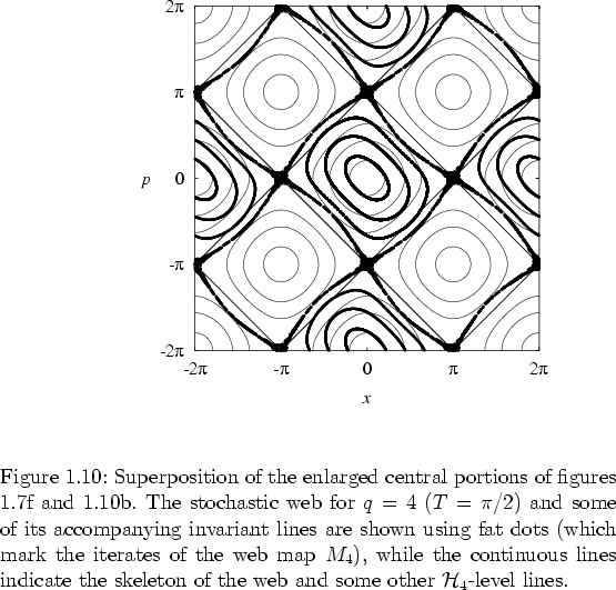
The quasiperiodic regular dynamics
in the meshes of the web, depicted in figure 1.7f, is
also (more or less) well approximated by the contour lines of
tends to zero, and accordingly the stochastic
webs more and more approach the rectangular grid of figure
1.10b.
The quasiperiodic regular dynamics
in the meshes of the web, depicted in figure 1.7f, is
also (more or less) well approximated by the contour lines of
![]() , as can be seen
in figure 1.12, where magnifications of figures 1.7f
and 1.10b have been superimposed.
, as can be seen
in figure 1.12, where magnifications of figures 1.7f
and 1.10b have been superimposed.
In contrast to the inevitably
qualitative description of the
symmetry of the stochastic webs displayed in figures 1.3a and
1.7/1.8,
the symmetry groups of the
skeletons
of the webs can be determined
exactly, because with equation (1.43) a closed formula for
the pattern they are forming is available.
For the skeleton of stochastic webs with ![]() (figure 1.10b),
the symmetry group is
(figure 1.10b),
the symmetry group is ![]() (using the ``international notation'' for planar space groups
[GS87]).
It is characterized by two classes of 4-fold rotation symmetries
(here: the centres of rotation being the elliptic points
(using the ``international notation'' for planar space groups
[GS87]).
It is characterized by two classes of 4-fold rotation symmetries
(here: the centres of rotation being the elliptic points
![]() ,
, ![]() even, in the centres of the meshes and the points
of channel crossings:
even, in the centres of the meshes and the points
of channel crossings: ![]() ,
, ![]() odd)
and a class of 2-fold rotation symmetries
(rotations about
odd)
and a class of 2-fold rotation symmetries
(rotations about
![]() ), in addition to the obvious
translation and (glide) reflection symmetries.
), in addition to the obvious
translation and (glide) reflection symmetries.
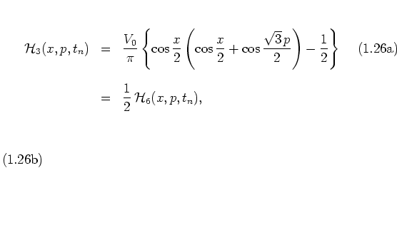
Some short remarks about the other values of
![]() might be in order.
Equation (1.43) again illustrates the triviality of the
cases
might be in order.
Equation (1.43) again illustrates the triviality of the
cases ![]() and
and ![]() (
(![]() and
and ![]() ).
For these
).
For these ![]() there is no
there is no ![]() -dependence any more and
-dependence any more and
![\begin{subequations}
\begin{eqnarray}
{\mathcal H}_1(x,p,t_n) & = & \frac{V_0}{...
...]
& = & \frac{1}{2} \, {\mathcal H}_2(x,p,t_n)
\end{eqnarray}\end{subequations}](img205.png)
such that the phase space structures effectively become one-dimensional
rather than two-dimensional,
as already discussed in the previous subsection
and displayed in figure 1.9.
Similarly, ![]() and
and ![]() (
(![]() and
and ![]() ) are also
intertwined with each other,
) are also
intertwined with each other,
and thus yield the same web skeleton, namely the level lines given by
![]() :
:
see figure 1.10a.
The symmetry group of this skeleton is ![]() and includes three classes of rotational symmetries, namely a
2-fold, a 3-fold and a 6-fold rotational symmetry (the rotations are
about the vertices and the centres of the triangles, and about the centres
of the hexagons in figure 1.10a, respectively),
in addition to the obvious translation and (glide) reflection symmetries.
and includes three classes of rotational symmetries, namely a
2-fold, a 3-fold and a 6-fold rotational symmetry (the rotations are
about the vertices and the centres of the triangles, and about the centres
of the hexagons in figure 1.10a, respectively),
in addition to the obvious translation and (glide) reflection symmetries.
The skeletons for
![]() show a more complicated structure.
In figures 1.11a and 1.11b
contours for a single
show a more complicated structure.
In figures 1.11a and 1.11b
contours for a single
![]() -level each are
shown; these levels are chosen in such a way that the contour lines
cover as many hyperbolic points in the stochastic layer as possible,
thereby coming fairly close to the underlying separatrix
(cf. [ZSUC88]).
Here, as in figure 1.3b, the aperiodic organization of phase
space is clearly visible.
-level each are
shown; these levels are chosen in such a way that the contour lines
cover as many hyperbolic points in the stochastic layer as possible,
thereby coming fairly close to the underlying separatrix
(cf. [ZSUC88]).
Here, as in figure 1.3b, the aperiodic organization of phase
space is clearly visible.
Essentially, the method I have used here to identify the webs' skeletons
is an averaging procedure
(see the derivation of the splitting (1.39)).
LOWENSTEIN [Low92] shows that this can be viewed as
just the first step of an iterative scheme which is similar to the
BIRKHOFF-GUSTAVSON normalization method
[Gus66,Eng93,ESE95]
and, step by
step, yields higher order
approximations
for
the Hamiltonian (1.17). Using this scheme it is
possible to systematically derive improved expressions describing the
separatrices of the webs and thereby explain their
waviness
that develops for
larger values
of ![]() , as can be
observed,
for example, in
figure 1.8.
, as can be
observed,
for example, in
figure 1.8.