Next: Diffusive Energy Growth in
Up: The Stochastic Web
Previous: The Skeleton of the
Contents
The Influence of the Kick Amplitude
In this subsection I demonstrate the influence of the kick amplitude  for the case
  ; similar results can be obtained for
  and
and
 . The following discussion holds for small values of .
The idea is to derive a separatrix mapping that describes the
dynamics of the kicked harmonic oscillator in the vicinity of the
separatrices and allows to estimate the width of the channels of diffusive
dynamics.
. The following discussion holds for small values of .
The idea is to derive a separatrix mapping that describes the
dynamics of the kicked harmonic oscillator in the vicinity of the
separatrices and allows to estimate the width of the channels of diffusive
dynamics.
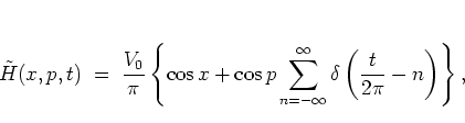
The first step is to identify
the
 of equation (1.39c) as a
high frequency perturbation to the time averaged Hamiltonian
of equation (1.39c) as a
high frequency perturbation to the time averaged Hamiltonian
 (1.44).
At kick times
(1.44).
At kick times
 ,
,
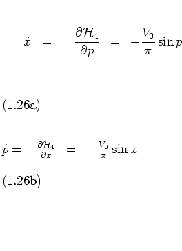
 , one has
 |
(1.25) |
which gives, with the help of equations (1.35),
for every fourth kick ( ,
,
 )
)
such that the action-angle variables  have been exchanged
for the original
have been exchanged
for the original  . now takes the form
 |
(1.26) |
which holds for every fourth kick time
 only.
This is
a useful feature of equation
(1.50), as it facilitates the discussion of the dynamics near
one of the four separatrices enclosing each phase space cell,
rather than near all four of them:
while for the dynamics of the web map
only.
This is
a useful feature of equation
(1.50), as it facilitates the discussion of the dynamics near
one of the four separatrices enclosing each phase space cell,
rather than near all four of them:
while for the dynamics of the web map  , corresponding to the full
Hamiltonian (1.17), it takes four iterates to
return into the neighbourhood of an initial value near a separatrix, the same neighbourhood
is reached by a single iteration of
, corresponding to the full
Hamiltonian (1.17), it takes four iterates to
return into the neighbourhood of an initial value near a separatrix, the same neighbourhood
is reached by a single iteration of  , or equivalently by the
discrete dynamics generated
by the Hamiltonian
, or equivalently by the
discrete dynamics generated
by the Hamiltonian
 , where in the form (1.50) is
used.
, where in the form (1.50) is
used.
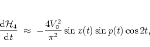
From the last formula
it becomes clear that can indeed be
treated as a high frequency perturbation of
the HARPER Hamiltonian
:
the time dependence of
is given by cosine terms
the largest period of which is  , whereas the smallest period
of
is
, whereas the smallest period
of
is
 -- as
is
shown below on page
-- as
is
shown below on page ![[*]](crossref.png) --
and can thus be made as
large
as desired in the limit
--
and can thus be made as
large
as desired in the limit  .
.
In [LL73] it is argued
that in a first approximation
the higher frequency terms of
a perturbation expanded as in equation (1.50)
can be neglected, although
they contribute with
roughly
the same
weight
( ) as the small frequency terms.
Therefore I can drop all cosine terms with
) as the small frequency terms.
Therefore I can drop all cosine terms with  and get the
approximant
and get the
approximant
 |
(1.27) |
where it turns out to be useful to keep the explicit  -dependence,
although strictly speaking this formula applies for
-dependence,
although strictly speaking this formula applies for  only.
only.
Now consider
a typical orbit of the web map in the stochastic region of the
web. For some
 the corresponding orbit point
  will be close to and just below of the midpoint of the
HARPER separatrix
will be close to and just below of the midpoint of the
HARPER separatrix  with
with  ,
which is displayed in the upper right quadrant of
figure 1.13.1.7
,
which is displayed in the upper right quadrant of
figure 1.13.1.7
For notational convenience I define
 with some
 .
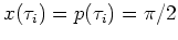
At
.
At
 ,
takes on
a certain value
,
takes on
a certain value
 since the
separatrices are characterized by
since the
separatrices are characterized by
 . Let be the initial
value (at time
. Let be the initial
value (at time  ) for the successive application of the fourth
iterate of the iteration of the web map (1.29), .
The resulting orbit in the
) for the successive application of the fourth
iterate of the iteration of the web map (1.29), .
The resulting orbit in the
 -plane
is quasiperiodic if is not
too near to the separatrix (cf. figure 1.7f). First the orbit
follows the separatrix anticlockwise, until it comes close
enough to the
hyperbolic point
-plane
is quasiperiodic if is not
too near to the separatrix (cf. figure 1.7f). First the orbit
follows the separatrix anticlockwise, until it comes close
enough to the
hyperbolic point  ,
where the orbit
turns left
and follows the
perpendicular separatrix
,
where the orbit
turns left
and follows the
perpendicular separatrix  with
with  ; this is shown
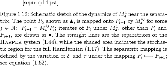
schematically in figure 1.14.
At some time
; this is shown
schematically in figure 1.14.
At some time
 (where
  is the according number of iterations of )
the orbit reaches
the point
is the according number of iterations of )
the orbit reaches
the point
 ,
which is defined as that iterate of under
that comes closest to the centre of the second separatrix.
This point again gives rise to a certain value of
,
,
which is defined as that iterate of under
that comes closest to the centre of the second separatrix.
This point again gives rise to a certain value of
,
 .
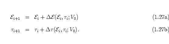
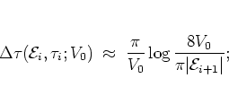
The desired separatrix mapping is now given by the change of the value of
during one such quarter revolution and by the corresponding
(approximate) quarter period:
.
The desired separatrix mapping is now given by the change of the value of
during one such quarter revolution and by the corresponding
(approximate) quarter period:
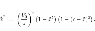
In order to determine an approximate expression for
 , I first derive an explicit solution of the
HARPER dynamics
, I first derive an explicit solution of the
HARPER dynamics
on the separatrix  for . Such a solution is given by
![\begin{displaymath}
\begin{array}{lcl}
x(t) & = & \displaystyle 2\arctan\exp\l...
...(t-\tau_i)}\right)\\ [0.5cm]
p(t) & = & \pi-x(t),
\end{array}\end{displaymath}](img252.png) |
(1.26) |
where
is
chosen
in such a way that
 ,
corresponding to the midpoint of the separatrix.
In figure 1.13 the corresponding trajectory connects the
limiting points
,
corresponding to the midpoint of the separatrix.
In figure 1.13 the corresponding trajectory connects the
limiting points
 and of the separatrix, for going from

to  .
.
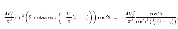
The rate of change of the value of
during the
-perturbed dynamics can then approximately be
calculated
as
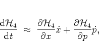 |
(1.27) |
where the partial derivatives
are to
be taken from equations
(1.53),
and
 stem from the Hamiltonian equations according to
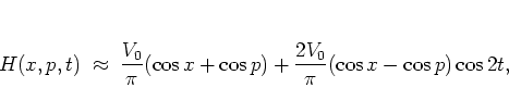 |
(1.28) |
which is used as an approximant to the full Hamiltonian (1.17)
at times  .
This gives
.
This gives
 |
(1.29) |
which holds for all  ,
, again.
Using the solution (1.54) for
,
, again.
Using the solution (1.54) for  and
and  , the right hand
side of equation (1.57) can be
approximated by
, the right hand
side of equation (1.57) can be
approximated by
such that by integration along the whole separatrix I finally
obtain1.8
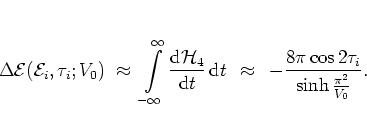 |
(1.31) |
Thus, while an exact formula for
certainly depends on
 ,
in the framework of this first approximation
is
independent of
.
,
in the framework of this first approximation
is
independent of
.
It remains to determine the time interval  in equation
(1.52b).
Within the cells, i.e. away from the separatrices, the equations of
motion of the unperturbed HARPER system
can be integrated using
Jacobian
elliptic functions.
With
in equation
(1.52b).
Within the cells, i.e. away from the separatrices, the equations of
motion of the unperturbed HARPER system
can be integrated using
Jacobian
elliptic functions.
With
 |
(1.32) |
which remains constant on each integral curve of the HARPER
system, and
 |
(1.33) |
equation (1.53a) can be transformed into
 |
(1.34) |
This is essentially the characteristic differential equation satisfied
by the elliptic function
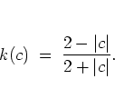
 [DV73], where the parameter
 is determined by the value of c:
 |
(1.35) |
With  the solution of the characteristic equation gives
![\begin{displaymath}
\begin{array}{lcl}
\cos x(t) & = & \displaystyle \frac{c}{...
...ad c\gl 0 \\ [0.5cm]
\cos p(t) & = & c-\cos x(t).
\end{array}\end{displaymath}](img280.png) |
(1.36) |
For real arguments,
as in the present case,
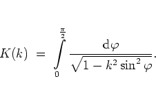
is periodic with period  ,
,  being a
complete elliptic integral of the first kind:
being a
complete elliptic integral of the first kind:
 |
(1.37) |
This integral is bounded below by
 . (The value
corresponds to the case
. (The value
corresponds to the case  , characterizing the centres of the phase
space cells.)
Therefore the period of the HARPER solution
, characterizing the centres of the phase
space cells.)
Therefore the period of the HARPER solution
 ,1.9
,1.9
 |
(1.38) |
is not smaller than
,
which tends to infinity for .
This justifies the above treatment of as a
high frequency perturbation of
(see pages f).
Approximate expressions for the integral (1.65) can be found
in [AS72] and yield here, in the vicinity of a
separatrix:
 |
(1.39) |
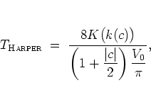
Taking into account that for the separatrix mapping only a quarter of a
full revolution has to be considered, equations (1.66)
and (1.67) finally give the desired expression for
,
 |
(1.40) |
when solving the upcoming equation (1.71) it turns out
that it is technically more convenient to use
here as a
replacement for  rather than
.
The
- and -dependence in this formula comes from
rather than
.
The
- and -dependence in this formula comes from
 -- see equations (1.52a) and
(1.59).
-- see equations (1.52a) and
(1.59).
With equations (1.59) and (1.68),
the separatrix mapping (1.52), approximating the dynamics of
near the separatrices, is completely specified.
Note that
the
separatrix mapping can also be obtained in a different way:
up to terms of order  , the fourth iterate of the web map
(1.29) is given by
, the fourth iterate of the web map
(1.29) is given by
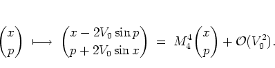 |
(1.41) |
This
map
can be generated using the kicked HARPER
Hamiltonian
 |
(1.42) |
which finds its application in solid state physics, for example in the
theory of electrons in
certain
magnetic fields
[KSD92,Dan95,FGKP95],
alongside its unkicked counterpart, the HARPER Hamiltonian
.
Submitting  to manipulations similar to those of the present
subsection, formulae (1.59) and (1.68) can be derived
once
again.
to manipulations similar to those of the present
subsection, formulae (1.59) and (1.68) can be derived
once
again.
Using the separatrix mapping, I now can proceed
to the estimation of the width of the channels of diffusive dynamics.
As a criterion for the
border between regular dynamics within the meshes
and stochastic dynamics in the channels,
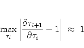 |
(1.43) |
may be used, since this expression
characterizes
the region of phase space where the value of begins to change
significantly under iteration of the separatrix mapping.
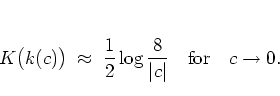
Solving relation (1.71) for
 and renaming it
 ,
I get
,
I get
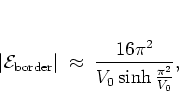 |
(1.44) |
such that with equation (1.44) I finally obtain for the width  of
the channels:
of
the channels:
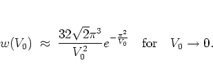 |
(1.45) |
This expression
scales with
 and, not surprisingly, tends to zero
in the limit .
and, not surprisingly, tends to zero
in the limit .
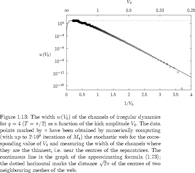
Figure 1.15 illustrates this behaviour: for several
values of stochastic webs are obtained numerically by iterating the
web map for a large number of times;
then the channel widths of these webs are measured
-- by determining the largest distance of any two points of the web
which approximately lie on the line  and near the point
 -- and compared with the numbers given by the approximating formula
(1.73).
The agreement between the analytical formula
-- and compared with the numbers given by the approximating formula
(1.73).
The agreement between the analytical formula
and the numerical data is reasonably good for
![$V_0 {\protect\begin{array}{c}
<\protect\\ [-0.3cm]\sim
\protect\end{array}} 1$](img308.png)
and improves for . Figure 1.15 also indicates
that for
![$V_0 {\protect\begin{array}{c}
<\protect\\ [-0.3cm]\sim
\protect\end{array}} 0.3$](img309.png)
the precision of the computer
algorithm
does not suffice any more to produce accurate numerical results,
because in this parameter range the web gets very thin
-- the width of the channels
shrinks to less than
 here.
Similar results hold for the other values of
here.
Similar results hold for the other values of
 .
.
In this subsection I have discussed how the kick strength of the
kicked harmonic oscillator determines the shape of its phase portrait.
In particular it has been shown that the periodic kicking acts in a way
which is typical for perturbed systems: starting from an integrable
system at  (here: the harmonic oscillator)
the kicking
(with
(here: the harmonic oscillator)
the kicking
(with  )
renders the
system nonintegrable,
and the
area
of the phase space region of irregular, chaotic dynamics
grows with increasing perturbation parameter .
)
renders the
system nonintegrable,
and the
area
of the phase space region of irregular, chaotic dynamics
grows with increasing perturbation parameter .
Having investigated the shape and the size of the channels of
irregular motion
in this subsection and the previous one, in the next subsection I turn to
the discussion of the most characteristic dynamical aspect of the
irregular motion.
Footnotes
- ...HarperDynamics.1.7
-
Any other separatrix
 with
with
 and
and
 could be
considered
as well. It depends on the choice of
and
could be
considered
as well. It depends on the choice of
and  whether
the rotation is clockwise or anticlockwise. The cell
centred around the origin of the
-plane
exhibits anticlockwise
rotation, and neighbouring cells have opposite directions of revolution.
See figure 1.13.
whether
the rotation is clockwise or anticlockwise. The cell
centred around the origin of the
-plane
exhibits anticlockwise
rotation, and neighbouring cells have opposite directions of revolution.
See figure 1.13.
- ...
obtain1.8
-
More explicitly,
has to be calculated in two steps:
first one integrates along the separatrix from
 to
to
 ;
then the perpendicular separatrix
;
then the perpendicular separatrix  is followed from to
 .
A closer investigation shows that this procedure can be replaced by
integrating along from
.
A closer investigation shows that this procedure can be replaced by
integrating along from  up to ; this corresponds
to the time integral from to using the on-separatrix
solution (1.54), as in equation (1.59).
up to ; this corresponds
to the time integral from to using the on-separatrix
solution (1.54), as in equation (1.59).
- ...,1.9
-
Note that the period of
 is twice the period of
 ,
,  .
.
Next: Diffusive Energy Growth in
Up: The Stochastic Web
Previous: The Skeleton of the
Contents
Martin Engel 2004-01-01
![\begin{figure}
% latex2html id marker 2694
\vspace*{-0.4cm}
\par
\hspace*{1.2cm}...
...continuation of the
% depicted
shown
interval $[-\pi,\pi]^2$.
}
\end{figure}](img233.png)