Next: ANDERSON Localization on One-dimensional
Up: ANDERSON Localization in the
Previous: ANDERSON Localization in the
Contents
The Kicked Rotor
The kicked rotor is one of the most frequently studied model systems in
dynamical systems theory. It emerges in many physical systems
(see for example [Zas85,MRB+95]),
and despite being very simple it has successfully been used
for modelling the onset of chaos, retaining many of the typical and
complex features of the underlying
physical
system.
After suitable scaling,
leading to dimensionless variables,
the kicked rotor can be defined by the
Hamiltonian
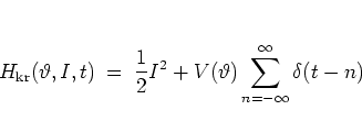 |
(5.1) |
with the angular displacement  and the angular momentum
  conjugate to .
In the present subsection I choose the kick potential
in the conventional way,
conjugate to .
In the present subsection I choose the kick potential
in the conventional way,
 |
(5.2) |
such that
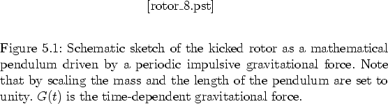
 models, for example, a mathematical pendulum
that is driven by ``impulsively acting gravity''
[CCIF79,LL92].
The first summand
models, for example, a mathematical pendulum
that is driven by ``impulsively acting gravity''
[CCIF79,LL92].
The first summand
 of describes free
rotation; the second specifies the periodic
``gravitational''
kicks the
strength of which depends on the
kick function.
See figure 5.1 for a schematic illustration.
In subsection 5.1.3 other
kick functions
are considered as well.
of describes free
rotation; the second specifies the periodic
``gravitational''
kicks the
strength of which depends on the
kick function.
See figure 5.1 for a schematic illustration.
In subsection 5.1.3 other
kick functions
are considered as well.
Note that while the Hamiltonian (5.1)
with the harmonic forcing (5.2)
is similar
to the Hamiltonian (1.17) of the kicked harmonic oscillator there
are two essential
differences:
the phase space of the rotor is a cylinder -- as opposed to the phase
plane of the oscillator --
and there is no harmonic potential term like
 in
.
Notice further that the rotor depends on the single parameter
in
.
Notice further that the rotor depends on the single parameter  only
that controls the amplitude of the kicks. This is in contrast to the
oscillator, where a second parameter (for example the period
only
that controls the amplitude of the kicks. This is in contrast to the
oscillator, where a second parameter (for example the period  of the
kicks) cannot be eliminated by scaling.
As I
outline
below these seemingly minor differences account for remarkably different
dynamics of the two model systems,
both in classical and quantum mechanics.
of the
kicks) cannot be eliminated by scaling.
As I
outline
below these seemingly minor differences account for remarkably different
dynamics of the two model systems,
both in classical and quantum mechanics.
Defining  ,
,  as the values of ,
immediately before the
as the values of ,
immediately before the  -th kick,
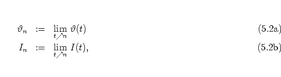
one obtains from the discrete time dynamics
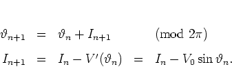 |
(5.2) |
This is the CHIRIKOV-TAYLOR map [Chi79]
or standard map.5.1The behaviour of this
discrete dynamical system
has been studied extensively in the literature
[Sch89,LL92] (the
second reference
contains a long
list of references on the
standard map).
The bifurcation scenario of this map for increasing values of
is a typical KAM scenario in the sense that,
as is increased, more and more invariant tori,
guaranteed to exist by the KAM theorem [GH83],
are destroyed.
Some phase portraits --
periodic with period  both in the
- and -directions -- of this transition to chaos are shown
in figure 5.2.
both in the
- and -directions -- of this transition to chaos are shown
in figure 5.2.
Figure 5.3:
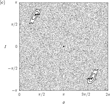
Figure 5.2: (continued)
(c)  . The initial value at
 is iterated 50000 times.
 |
For  (figure 5.2a) the phase portrait is
dominated by
the
invariant lines
of regular dynamics.
For the intermediate parameter value
(figure 5.2a) the phase portrait is
dominated by
the
invariant lines
of regular dynamics.
For the intermediate parameter value  (figure 5.2b) the regime of weak chaos has
been reached where invariant lines, POINCARÉ-BIRKHOFF island chains and
chaotic regions coexist.
For large enough unbounded motion in
the
direction of becomes
possible: at a critical value
(figure 5.2b) the regime of weak chaos has
been reached where invariant lines, POINCARÉ-BIRKHOFF island chains and
chaotic regions coexist.
For large enough unbounded motion in
the
direction of becomes
possible: at a critical value
 only a single global torus -- the
``golden'' KAM torus -- persists, and for
only a single global torus -- the
``golden'' KAM torus -- persists, and for
 it is destroyed, giving way for global diffusion in phase space
(figure 5.2c, for ).
it is destroyed, giving way for global diffusion in phase space
(figure 5.2c, for ).
Energy diffusion of the rotor
in the classical  -phase space can be described by
considering the rotational energy5.2before the -th kick:
-phase space can be described by
considering the rotational energy5.2before the -th kick:
 |
(5.3) |
The standard map (5.4) makes  evolve according to
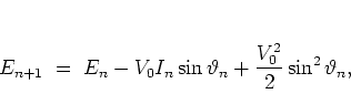 |
(5.4) |
which by averaging over an ensemble of orbits and employing the random
phase approximation (cf. subsection 1.2.4) becomes the
diffusion law
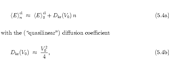
such that normally diffusive dynamics is to be expected.
This averaging is justified for large enough , when unhindered
diffusion through phase space is possible.
Corrections to formula (5.7b) resulting from accelerator modes
and angular correlations are discussed in [LL92],
for example.
In analogy with the quantum map of the kicked harmonic oscillator
introduced in section 2.1,
the quantum dynamics of the kicked rotor is
given by
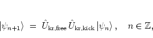 |
(5.4) |
with the quantum state
 just before the -th kick,
 |
(5.5) |
and the
time evolution operators
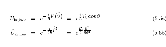
for the kick and the unperturbed dynamics, respectively, where
 and
and  are the angle and
angular momentum operators,
and
are the angle and
angular momentum operators,
and
 is the potential energy operator.
Unlike the classical system that contains the single parameter
only, the quantum system depends on both the parameters and
is the potential energy operator.
Unlike the classical system that contains the single parameter
only, the quantum system depends on both the parameters and
 .
The dependence on
is essential for the proof of quantum localization in
subsection 5.1.3
below.
.
The dependence on
is essential for the proof of quantum localization in
subsection 5.1.3
below.
The quantum map (5.8) can be iterated
comparatively easily
since the unperturbed dynamics of the rotor is
free rotation and the propagator
 becomes a mere multiplication operator in the
angular momentum representation: for
expanded according to
becomes a mere multiplication operator in the
angular momentum representation: for
expanded according to
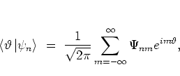 |
(5.5) |
using the FOURIER coefficients
![$\Psi_{nm} = \rule[-0.1cm]{0.0cm}{0.1cm}_{\rm r}\!\left< m \left\vert \psi_n \right> \right.$](img909.png) with
the eigenstates of angular momentum
with
the eigenstates of angular momentum
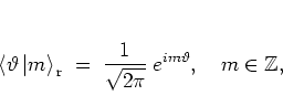 |
(5.6) |
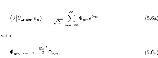
with respect to the eigenvalues  ,
one obtains for the free rotation part of the dynamics:
,
one obtains for the free rotation part of the dynamics:
Switching between the angle and angular
momentum representations can be accomplished with little numerical effort
by fast FOURIER transformation
(cf. the footnote on page ![[*]](crossref.png) ).
This makes the kicked rotor a numerically much
more accessible model than the kicked
harmonic
oscillator, where the quantum map
typically has to be iterated by multiplying with huge matrices,
as described in
chapter 3.
In [CCIF79] another numerical method for iterating
the quantum map of the cosine-kicked rotor is described, which is even
more efficient than the FFT-based method, but
has
the disadvantage
of being less general because it is tailored to the special kick potential
(5.2).
).
This makes the kicked rotor a numerically much
more accessible model than the kicked
harmonic
oscillator, where the quantum map
typically has to be iterated by multiplying with huge matrices,
as described in
chapter 3.
In [CCIF79] another numerical method for iterating
the quantum map of the cosine-kicked rotor is described, which is even
more efficient than the FFT-based method, but
has
the disadvantage
of being less general because it is tailored to the special kick potential
(5.2).
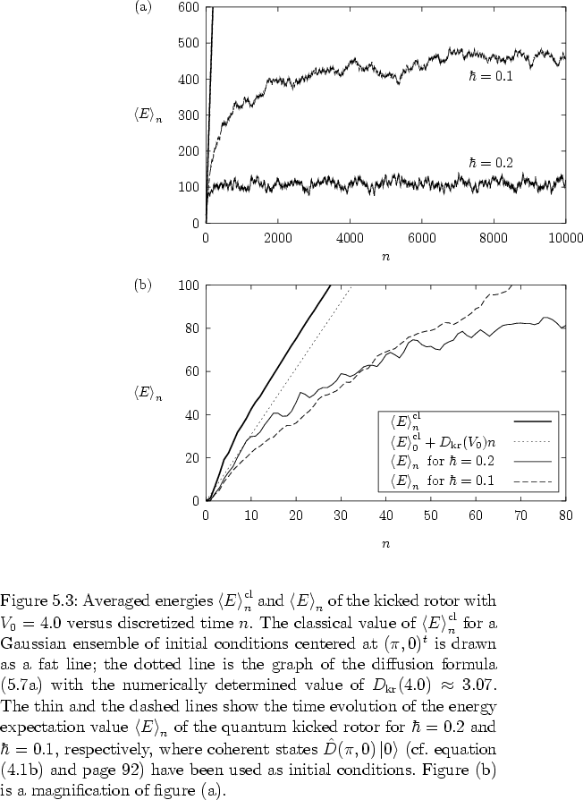
Results of numerical experiments for both the classical and quantum
rotors are shown in figure 5.4, where classical
normal diffusion in the case  is contrasted with
quantum mechanically suppressed diffusion.
is contrasted with
quantum mechanically suppressed diffusion.
The classical diffusion
coefficient is found numerically as
 , a somewhat smaller value than given by the
large approximation (5.7b), due to the small value
of
(cf. the discussion, at the end of subsection 1.2.4,
of a similar situation with respect to the kicked harmonic oscillator).
On the other hand, the quantum energy expectation value as a
function of
discretized time ,
, a somewhat smaller value than given by the
large approximation (5.7b), due to the small value
of
(cf. the discussion, at the end of subsection 1.2.4,
of a similar situation with respect to the kicked harmonic oscillator).
On the other hand, the quantum energy expectation value as a
function of
discretized time ,
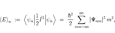 |
(5.6) |
exhibits a notably distinct behaviour.
Up to a quantum break time  ,
,
 follows the classical curve (5.7a), but
is suppressed for larger times;
even
appears
to be bounded
for all .
(In the present example one has
follows the classical curve (5.7a), but
is suppressed for larger times;
even
appears
to be bounded
for all .
(In the present example one has
 for
for  and
and  for
for  ;
but note that these values of
are subject not only to the value of , but also depend on and
the initial state
;
but note that these values of
are subject not only to the value of , but also depend on and
the initial state
 .)
.)
It is this
quantum mechanically suppressed energy diffusion, or
quantum localization, of the
kicked rotor that is
to be explained in the following two subsections.
Footnotes
- ... map.5.1
-
The sign of
the force term
in
the standard map
(5.4)
or in the potential (5.2)
is a matter of convention.
Changing this sign is equivalent to
shifting by
 .
.
- ... energy5.2
-
Due to the boundedness of the rotor's phase space
in the direction
of
,
energy
diffusion occurs only in the (angular) momentum
coordinate here,
as opposed to the case of the kicked harmonic oscillator, where both the
position and momentum variables
 ,
,  are unbounded
and
subject to diffusion
-- cf. equations (1.74, 1.77).
are unbounded
and
subject to diffusion
-- cf. equations (1.74, 1.77).
Next: ANDERSON Localization on One-dimensional
Up: ANDERSON Localization in the
Previous: ANDERSON Localization in the
Contents
Martin Engel 2004-01-01