The classical stochastic webs discussed in chapter 1 are objects within classical phase space, which is spanned by both the position and momentum variables. This is an inherently classical concept, as in quantum mechanics either the position or the momentum representation can be used, but these representations are mutually exclusive. Therefore it is not a priori clear how the classical and quantum results are to be compared.
A solution for this problem of
classical-quantum comparison
is to consider quantum phase space distribution functions.
In appendix A I describe in some detail how such
distributions can be defined and used to compare a quantum state with a
classical phase portrait. It turns out that many different phase space
distributions can be defined, but the most important is the
HUSIMI distribution
![]() .
In many respects, this
quasiprobability distribution function
is as close
as possible
to the
(LIOUVILLE) probability distributions in phase space
obtained for classical systems.
In the same way as
.
In many respects, this
quasiprobability distribution function
is as close
as possible
to the
(LIOUVILLE) probability distributions in phase space
obtained for classical systems.
In the same way as
![]() in the position representation
contains exactly the same information
as
in the position representation
contains exactly the same information
as
![]() in the momentum representation,
in the momentum representation,
![]() gives an equivalent description of the
quantum state
gives an equivalent description of the
quantum state
![]() .
.
![]() is a numerical parameter that can be chosen as desired;
here I use
is a numerical parameter that can be chosen as desired;
here I use ![]() alone, in which case the HUSIMI distribution is
also known as the coherent state representation.
See appendix A for more
information
on the theory of quantum phase distribution functions.
alone, in which case the HUSIMI distribution is
also known as the coherent state representation.
See appendix A for more
information
on the theory of quantum phase distribution functions.
I now begin the discussion of the numerical methods with the example of
![]() ,
, ![]() and the resonance given by
and the resonance given by ![]() (
(![]() ). This value
of
). This value
of ![]() classically leads to rectangular classical stochastic webs as shown
in figures
1.7, 1.8, 1.10b and 1.12.
The skeletons
of the classical stochastic webs for
classically leads to rectangular classical stochastic webs as shown
in figures
1.7, 1.8, 1.10b and 1.12.
The skeletons
of the classical stochastic webs for ![]() are given by the square grid (1.45).
In the figures of the present section
for
are given by the square grid (1.45).
In the figures of the present section
for ![]() , this grid is displayed via thin
lines, in addition to the contour lines of
, this grid is displayed via thin
lines, in addition to the contour lines of
![]() .
.
In figure 4.1,
the result of a numerical simulation is shown for which the GOLDBERG finite differences algorithm of subsection 3.1.2 has been used. In the interval
Using the parameters stated above, the harmonic oscillator representation
method runs
much faster than the finite differences method:
on a Pentium 4 with 2 GHz, the algorithms require approximately
10 sec / 150 sec per iteration of the quantum map, respectively.
After a closer inspection of the numerical data it also turns out that the
GOLDBERG algorithm produces a faster growing numerical error,
manifesting itself in an increasing deviation of the norm of the numerically
modelled quantum state from its nominal value of 1.
In principle, this error
can be controlled by adaptively using smaller time steps
![]() ,
but only at considerable numerical cost.
The second method
also produces a numerical error, but at a distinctly smaller rate: after
,
but only at considerable numerical cost.
The second method
also produces a numerical error, but at a distinctly smaller rate: after
![]() kicks, for example, the respective errors
of the two runs shown in the figures
are of the order of
kicks, for example, the respective errors
of the two runs shown in the figures
are of the order of
![]() and
and ![]() , respectively.
, respectively.
This is reflected in the figures:
the initial state
![]() --
the HUSIMI distribution corresponding to the ground state
--
the HUSIMI distribution corresponding to the ground state
![]() of the harmonic oscillator is a two-dimensional Gaussian in phase
space, centered around
of the harmonic oscillator is a two-dimensional Gaussian in phase
space, centered around ![]() ;
see figures
4.1 (
;
see figures
4.1 (![]() ),
4.2 (
),
4.2 (![]() ) and
A.1c --
evolves into a web-like structure, as the more exact figure
4.2 nicely shows.
The
spreading of the wave packet is visible in figure
4.1
as well, but there it takes place much more slowly and in a much less
pronounced fashion;
the periodic pattern clearly displayed in figure
4.2
evolves much more slowly in figure
4.1,
again indicating a numerical error of the GOLDBERG result. This
error could be reduced by increasing
) and
A.1c --
evolves into a web-like structure, as the more exact figure
4.2 nicely shows.
The
spreading of the wave packet is visible in figure
4.1
as well, but there it takes place much more slowly and in a much less
pronounced fashion;
the periodic pattern clearly displayed in figure
4.2
evolves much more slowly in figure
4.1,
again indicating a numerical error of the GOLDBERG result. This
error could be reduced by increasing
![]() and
and ![]() , and by
spending more numerical effort on solving equation
(3.21) in order to control cancellations and other
numerical errors; but in any case the method would be slowed down further.
, and by
spending more numerical effort on solving equation
(3.21) in order to control cancellations and other
numerical errors; but in any case the method would be slowed down further.
This behaviour of the GOLDBERG algorithm, suggesting that a considerably greater numerical effort has to be spent for obtaining sufficiently accurate results, has also been observed in several other calculations performed for other parameter combinations; it seems to be typical for this algorithm when applied to the quantum map of the kicked harmonic oscillator. Consequentially, the GOLDBERG algorithm is not used further on in this study. All the rest of the numerical iterations of the quantum map shown in chapters 4 and 5 and in appendix C have been carried out using the superior algorithm, namely the method using the propagator in the eigenrepresentation of the harmonic oscillator.
If the computation of the quantum analogues of stochastic webs had been
the only focus of this work, then using the GOLDBERG algorithm with
periodic boundary conditions (3.24b)
might have been an alternative approach, potentially faster in obtaining
the complete web than the
other methods, because periodicity in ![]() -direction is already
built
into the algorithm.
But this advantage is compensated by the disadvantage that solving
equation (3.21) becomes numerically more difficult for
periodic boundary conditions and
easily leads to cancellations, overflows etc.
In principle, these difficulties can be mastered
-- for example by solving equation (3.21) using
iterative methods like SOR (successive overrelaxation)
[SB00] --
but again only at considerable numerical cost for each iteration of the
quantum map.
-direction is already
built
into the algorithm.
But this advantage is compensated by the disadvantage that solving
equation (3.21) becomes numerically more difficult for
periodic boundary conditions and
easily leads to cancellations, overflows etc.
In principle, these difficulties can be mastered
-- for example by solving equation (3.21) using
iterative methods like SOR (successive overrelaxation)
[SB00] --
but again only at considerable numerical cost for each iteration of the
quantum map.
In addition to the better numerical performance, the harmonic oscillator eigenrepresentation method also has the advantage that the same numerical algorithm can be used for all three relevant cases, i.e. for periodic and aperiodic stochastic webs and for the case of nonresonance. Of these, only the periodic webs allow the application of an algorithm relying on periodic boundary conditions, whereas the method used here can cope with all three cases.
Although this algorithm runs comparably fast, while producing quite
accurate results, it should be noted
that the computer time needed for these simulations can be quite long.
As long as the achieved numerical accuracy allows it,
in the following
often the
long-time dynamics for up to ![]() kicks is
studied.
Typically, on a fast workstation, it takes up to and beyond ten days to
complete such a simulation run.
Series of simulations of this scope, where the parameters
kicks is
studied.
Typically, on a fast workstation, it takes up to and beyond ten days to
complete such a simulation run.
Series of simulations of this scope, where the parameters ![]() ,
, ![]() ,
,
![]() each take on several different values, can be
performed
only if a
larger number of fast workstations is available.
each take on several different values, can be
performed
only if a
larger number of fast workstations is available.
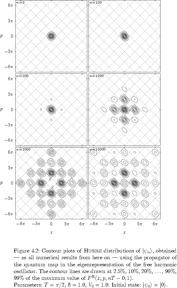
In figure
4.2,
the dynamics can be iterated up to roughly ![]() kicks, before the
cut-off error reduces the numerical norm of
kicks, before the
cut-off error reduces the numerical norm of
![]() too
much.
For
too
much.
For ![]() , the figure indicates that the HUSIMI distribution already
exhibits a nearly periodic pattern within the square grid shown.
Furthermore, the figure also suggests a 4-fold rotational symmetry,
just as for the classical stochastic webs
for
, the figure indicates that the HUSIMI distribution already
exhibits a nearly periodic pattern within the square grid shown.
Furthermore, the figure also suggests a 4-fold rotational symmetry,
just as for the classical stochastic webs
for ![]() .4.1
.4.1
![]() tends to be concentrated in the meshes
of the classical web, rather than in the channels, where the
-- classical and quantum mechanical --
phase space
density gets transported away along the classical skeleton
(1.45)
rapidly.
tends to be concentrated in the meshes
of the classical web, rather than in the channels, where the
-- classical and quantum mechanical --
phase space
density gets transported away along the classical skeleton
(1.45)
rapidly.
Figure 4.2 leads to the
conjecture that, as in the classical case, for ![]() the
web-like structure uniformly extends over the complete phase space and
thus establishes (the meshes of) the quantum stochastic web,
only the central portion of which is shown in
the figure.
The classical and the quantum stochastic webs for
the
web-like structure uniformly extends over the complete phase space and
thus establishes (the meshes of) the quantum stochastic web,
only the central portion of which is shown in
the figure.
The classical and the quantum stochastic webs for ![]() seem to be characterized by the same symmetries.
seem to be characterized by the same symmetries.
In figures
4.1 and
4.2,
an initial state
![]() corresponding to a HUSIMI distribution
centered in a mesh of the stochastic web has been
used, leading to a web-like structure which obviously is concentrated in
the meshes of the web.4.2This makes it natural to ask for an initial state that is located
somewhere in the channels of the web.
corresponding to a HUSIMI distribution
centered in a mesh of the stochastic web has been
used, leading to a web-like structure which obviously is concentrated in
the meshes of the web.4.2This makes it natural to ask for an initial state that is located
somewhere in the channels of the web.
To this end, WEYL's unitary displacement operator,
or translation operator,
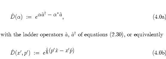
needs to be considered;
the parameters
![]() are essentially the real and
imaginary parts of
are essentially the real and
imaginary parts of
![]() :4.3
:4.3
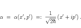
Using the translation operator, initial states like
 |
(4.1) |
For the following figures,
depending on the value of ![]() ,
,
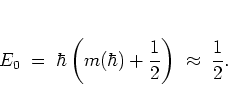
![]() in the initial states
in the initial states
![]() and
and
![]() is chosen in such a way
that the energy of
is chosen in such a way
that the energy of
![]() is as close to 1/2 as possible:
is as close to 1/2 as possible:
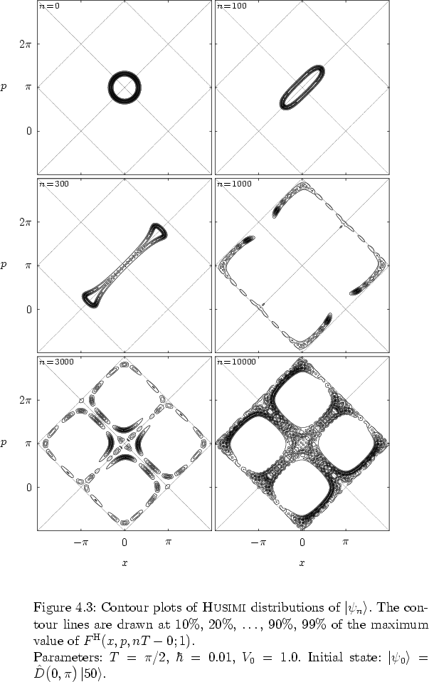
This formalism is applied for figure 4.3,
where for
Figure 4.3
convincingly shows how the
central portions of the stochastic web get filled by the
phase space density
evolving with time.
Iterating for more than the ![]() kicks shown in the figure, one would
also see that not only the central portion of the channels of the web
gets visited by the dynamics, but that later on the phase space density
to a larger degree
flows into the outer parts of the web, too.
(Because of the declining numerical accuracy at large
kicks shown in the figure, one would
also see that not only the central portion of the channels of the web
gets visited by the dynamics, but that later on the phase space density
to a larger degree
flows into the outer parts of the web, too.
(Because of the declining numerical accuracy at large ![]() for fixed
for fixed
![]() , such figures are not shown here.)
Note how closely the quantum web sticks to the square grid marking
the skeleton of the classical web. In this sense, the part of phase space
covered in figure 4.3
at
, such figures are not shown here.)
Note how closely the quantum web sticks to the square grid marking
the skeleton of the classical web. In this sense, the part of phase space
covered in figure 4.3
at ![]() -- plus its periodic continuation along the grid lines --
marks the skeleton of the quantum stochastic web.
-- plus its periodic continuation along the grid lines --
marks the skeleton of the quantum stochastic web.
It is also interesting to see how in this particular case
at least for some time
the quantum
dynamics quite closely mimics the classical
evolution of an
ensemble of phase space points: the figure for ![]() shows how the quantum distribution is stretched along the skeleton line
described by
shows how the quantum distribution is stretched along the skeleton line
described by ![]() , while being compressed
in the direction of
, while being compressed
in the direction of ![]() . This is just the classical behaviour
near the separatrices -- near the stable and unstable manifolds -- of
the fixed point
. This is just the classical behaviour
near the separatrices -- near the stable and unstable manifolds -- of
the fixed point ![]() (with respect to the mapping
(with respect to the mapping ![]() ; cf. equation (1.29)).
Similarly, the figures for
; cf. equation (1.29)).
Similarly, the figures for ![]() ,
, ![]() and
and ![]() demonstrate the
dynamics in the neighbourhood of other classical separatrices: the
quantum distribution roughly follows the unstable manifold of a
fixed point until it comes close enough to the next fixed point, where it
again changes direction, as
determined
by the respective separatrix.
Sections C.1 and
C.2 of the appendix contain
several additional examples where this behaviour can clearly be
recognized;
see for example figures
C.15,
C.17,
C.35 and
C.36.
demonstrate the
dynamics in the neighbourhood of other classical separatrices: the
quantum distribution roughly follows the unstable manifold of a
fixed point until it comes close enough to the next fixed point, where it
again changes direction, as
determined
by the respective separatrix.
Sections C.1 and
C.2 of the appendix contain
several additional examples where this behaviour can clearly be
recognized;
see for example figures
C.15,
C.17,
C.35 and
C.36.
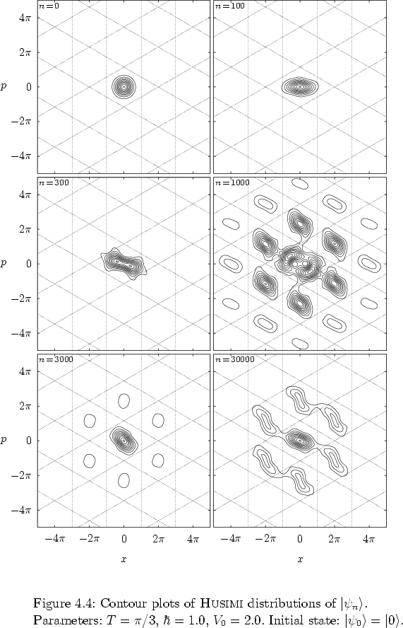
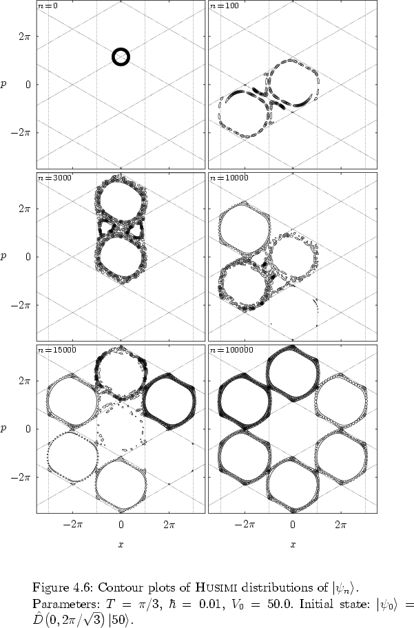
Similar HUSIMI contour plots, but for the resonance case ![]() (
(![]() ),
are displayed in figures
4.4-4.6.
),
are displayed in figures
4.4-4.6.
The 6-fold
(respectively 2-fold: cf. the footnote on page ![[*]](crossref.png) )
rotational symmetry of the quantum state shown in figure
4.4 becomes
clearly visible, once the quantum map is iterated often enough:
)
rotational symmetry of the quantum state shown in figure
4.4 becomes
clearly visible, once the quantum map is iterated often enough:
![$n{ {\protect\begin{array}{c}
>\protect\\ [-0.3cm]\sim
\protect\end{array}} }1000$](img695.png) . The picture for
. The picture for ![]() also gives a good
indication already of what the quantum web
would
look like for
also gives a good
indication already of what the quantum web
would
look like for
![]() .
.
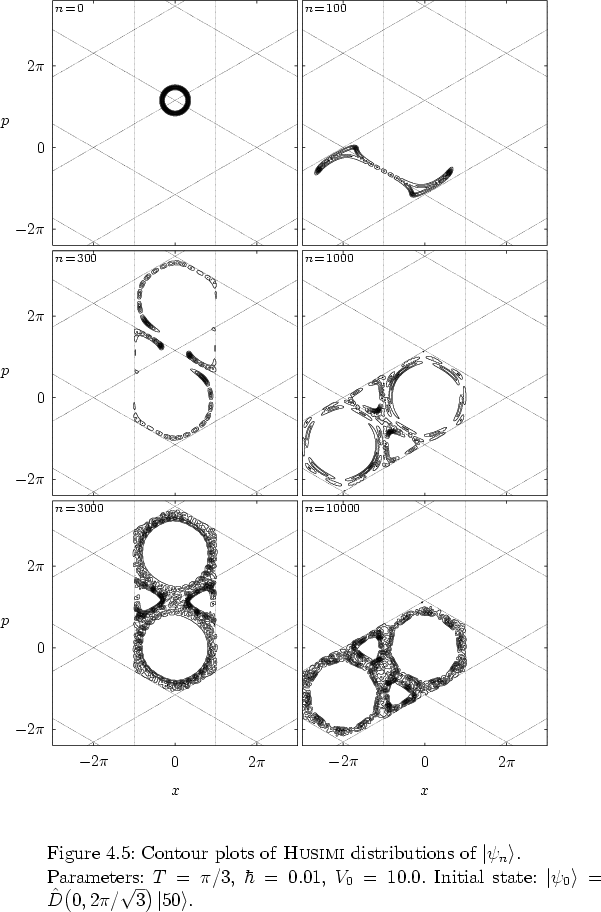
In figures 4.5 and 4.6, in addition to the usual level lines also the 2.5%-contours are plotted. In this way, for a suitably chosen initial state, the central portion of the channels of the web becomes densely filled by level lines after sufficiently large time, thereby exhibiting the stochastic region of the quantum stochastic web more clearly.
For all ![]() shown, the dynamics in figure
4.5
is obviously still in a transient stage.
While for growing
shown, the dynamics in figure
4.5
is obviously still in a transient stage.
While for growing ![]() the HUSIMI distributions spread more and more
in phase space, different phase space cells are visited one after the
other in a way that mimics the corresponding classical dynamics in a
periodic web: classically, for
the HUSIMI distributions spread more and more
in phase space, different phase space cells are visited one after the
other in a way that mimics the corresponding classical dynamics in a
periodic web: classically, for ![]() the iteration of the
web map (1.24) yields sequences of points that,
qualitatively speaking,
rapidly encircle the origin of phase space, completing
approximately one
rotation after every six iterations;
superimposed to this is the much slower component of
the dynamics in radial direction.
This quantum-classical mimicry leads to the
phase portraits in figure
4.5
being asymmetric with respect to 6-fold rotations around the origin of
phase space.
For values of
the iteration of the
web map (1.24) yields sequences of points that,
qualitatively speaking,
rapidly encircle the origin of phase space, completing
approximately one
rotation after every six iterations;
superimposed to this is the much slower component of
the dynamics in radial direction.
This quantum-classical mimicry leads to the
phase portraits in figure
4.5
being asymmetric with respect to 6-fold rotations around the origin of
phase space.
For values of ![]() exceeding
exceeding ![]() , the phase space distributions
can be expected to become more symmetric
-- in a way that is similar to the development of the web displayed in
the following figure.
, the phase space distributions
can be expected to become more symmetric
-- in a way that is similar to the development of the web displayed in
the following figure.
Finally, figure
4.6
is remarkable in that it shows
the way in which
a larger part of the quantum web
becomes explored in the course of the dynamics. For ![]() , the
phase portraits look similar to those of figure
4.5
and the phase space regions with essentially nonzero
, the
phase portraits look similar to those of figure
4.5
and the phase space regions with essentially nonzero
![]() are still approximately confined to only two
meshes of the web at any given time. For larger
times, though,
are still approximately confined to only two
meshes of the web at any given time. For larger
times, though,
![]() increasingly becomes distributed
over more than just two meshes, and it is natural to
assume that, for times larger than
increasingly becomes distributed
over more than just two meshes, and it is natural to
assume that, for times larger than ![]() ,
this process continues, comprising even more -- and finally all --
meshes of the web.
,
this process continues, comprising even more -- and finally all --
meshes of the web.
When the quantum map is iterated as often as ![]() , the question of
accuracy of the computed states needs to be addressed again.
After so many iterations, the numerical
, the question of
accuracy of the computed states needs to be addressed again.
After so many iterations, the numerical
![]() should not be
expected to
be exactly the state
should not be
expected to
be exactly the state
![]() . But in the spirit of the
Shadowing Lemma of dynamical systems theory [GH83],
one may hope that the sequence
. But in the spirit of the
Shadowing Lemma of dynamical systems theory [GH83],
one may hope that the sequence
![]() the computer finds
is nonetheless an approximation to some true quantum dynamics of the
system, presumably with respect to a somewhat different initial state
the computer finds
is nonetheless an approximation to some true quantum dynamics of the
system, presumably with respect to a somewhat different initial state
![]() .
Relying on this heuristic argument,
one can more or less safely iterate as long as desired,
provided the norms of the computed states do not deviate too much from 1.
.
Relying on this heuristic argument,
one can more or less safely iterate as long as desired,
provided the norms of the computed states do not deviate too much from 1.
Some more contour plots of quantum stochastic webs generated by the
quantum kicked harmonic oscillator for
![]() (
(![]() ),
), ![]() (
(![]() ) and
) and ![]() (
(![]() )
can be found in sections C.1,
C.2 and C.3 of the appendix.
)
can be found in sections C.1,
C.2 and C.3 of the appendix.
The portion of phase space significantly covered by the HUSIMI distribution can be visualized approximately by plotting the 1%-contour
lines of
![]() . For
. For ![]() ,
, ![]() ,
, ![]() and
and ![]() ,
this is done in
figure 4.7.
,
this is done in
figure 4.7.
![\begin{figure}
% latex2html id marker 10904
\par
\rule{0.0cm}{1.5cm}
\vspace*{-...
...0 \right>=\left\vert 0 \right>$.
%
\rule[-1.0cm]{0.0cm}{1.0cm}
}
\end{figure}](img648.png)
![\begin{figure}
% latex2html id marker 12772
\par
\rule{0.0cm}{0.3cm}
\vspace*{-...
...0,\pi\big)\left\vert 5 \right>$.
%
\rule[-1.0cm]{0.0cm}{1.0cm}
}
\end{figure}](img702.png)