


Next: Squeezed States
Up: Minimum Uncertainty States and
Previous: Minimum Uncertainty States and
Contents
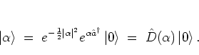
Coherent States
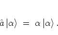
A coherent state
 is an eigenstate of the
annihilation operator
is an eigenstate of the
annihilation operator  with respect to the eigenvalue
 :
:
 |
(A.24) |
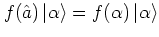
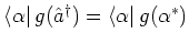
These states
are especially useful when dealing with
operators that are expanded in terms of the ladder operators
 ,
: an operator in this form can easily be applied to a coherent state
by treating as the c-number
,
: an operator in this form can easily be applied to a coherent state
by treating as the c-number  , i.e. by evaluating expressions of the form
 and
and
 . Situations like this are
frequently encountered in quantum optics.
An example for the
application of coherent states in this field is the modelling of
stationary vibrational states of a laser-driven ion in an ion trap
[DMFV96a,DMFV96b].
. Situations like this are
frequently encountered in quantum optics.
An example for the
application of coherent states in this field is the modelling of
stationary vibrational states of a laser-driven ion in an ion trap
[DMFV96a,DMFV96b].
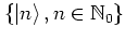
An explicit formula for coherent states can be found by expanding
in terms of the eigenstates of the harmonic oscillator, or
number states
 ,
,
 ,
substituting into
the definition
(A.34) and
equating the coefficients of the
. The result is
,
substituting into
the definition
(A.34) and
equating the coefficients of the
. The result is
 |
(A.25) |
for all
. Here, the factor
 is
chosen in such a way that
is normalized, since
for all
is
chosen in such a way that
is normalized, since
for all
 one has:
 |
(A.26) |
and therefore
 . Equations (A.34)
and (A.35) show that every
is an eigenvalue of
and thus defines a coherent state
.
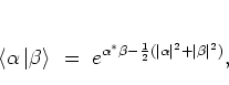
Note that the
are not pairwise orthogonal,
as the scalar product
. Equations (A.34)
and (A.35) show that every
is an eigenvalue of
and thus defines a coherent state
.
Note that the
are not pairwise orthogonal,
as the scalar product
 is not zero for
 .
.
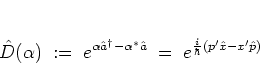
In order to come to a more intuitive understanding of coherent states
it is useful to consider WEYL's unitary
displacement operator
[MM71]
 |
(A.27) |
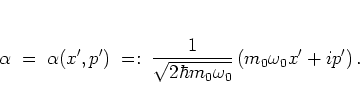
with the real parameters  and
and  , which are essentially the real and
imaginary parts of :
, which are essentially the real and
imaginary parts of :
 |
(A.28) |
Formally, is obtained from the definition of the annihilation
operator (A.24) by exchanging the operators  ,
,  for the scalars , .
As indicated by its name,
the displacement operator
acts on a state by shifting
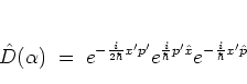
it in phase space. Using the BAKER-CAMPBELL-HAUSDORFF formula
(A.4) one can derive the product representation
 |
(A.29) |
of
 , which turns out to be the composition of the two
translation operators
, which turns out to be the composition of the two
translation operators
 and
and
 -- in addition to these there is also the phase
factor
-- in addition to these there is also the phase
factor
 which is irrelevant for the
interpretation of
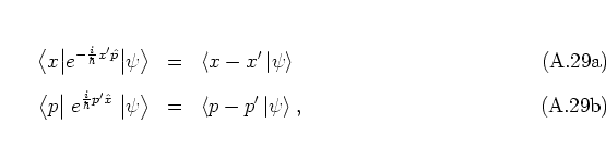
. The translation operators
each move
a wave packet in position and momentum space by and ,
respectively,
which is irrelevant for the
interpretation of
. The translation operators
each move
a wave packet in position and momentum space by and ,
respectively,
such that in phase space
 |
(A.29) |
moves the wave packet by the vector  .
The
translation operator
.
The
translation operator
 of equation
(A.11) is a special case of the more general
of equation
(A.11) is a special case of the more general
 :
:
 .
.
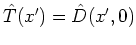
Using
the displacement operator
one can now write a coherent state as
 |
(A.30) |
This implies that all coherent states can be generated by
acting on the coherent state
defined by
 . This particular coherent state
 is identical
with the ground state
is identical
with the ground state
 of the harmonic oscillator, as can be
concluded from equation (A.35).
of the harmonic oscillator, as can be
concluded from equation (A.35).
With this result it is now clear how the set of all coherent states
 is to be interpreted:
it is obtained by
moving the ground state of the harmonic oscillator to all points of the
phase plane. Therefore the well-known properties of
,
is to be interpreted:
it is obtained by
moving the ground state of the harmonic oscillator to all points of the
phase plane. Therefore the well-known properties of
,
![\begin{displaymath}
\left< x \left\vert 0 \right> \right. \; = \; \sqrt[4]{\frac...
...2}
\quad \mbox{with} \quad
\sigma^2=\frac{\hbar}{m_0\omega_0}
\end{displaymath}](img1370.png) |
(A.31) |
(see equation (2.39)),
carry over to each of
the coherent states. With the parameters
,
of equation (A.38)
one then has for all states
:
![\begin{subequations}
\begin{eqnarray}
\big< {\hat{x}}\big> & = & x' \\ [0.2cm]...
... & \frac{1}{\sqrt{2}} \: \frac{\hbar}{\sigma}.
\end{eqnarray}\end{subequations}](img1371.png)
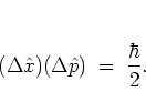
In particular, the coherent states are minimum uncertainty states,
i.e. they are characterized by the smallest possible product of
standard deviations of the position and momentum operators
as given by the HEISENBERG uncertainty relation:
 |
(A.31) |
In addition, setting  (for example by a suitable scaling as
in
section 2.1)
one obtains coherent states for which the
standard deviations of position and momentum are the same:
(for example by a suitable scaling as
in
section 2.1)
one obtains coherent states for which the
standard deviations of position and momentum are the same:
 |
(A.32) |
In the form (A.35) coherent states were first constructed by
SCHRÖDINGER, who
intended to use
them to demonstrate the ``continuous transition
from micro- to macromechanics'' [Sch26].
He showed that a wave packet (A.35), when specified as the
initial state submitted to the potential of the harmonic oscillator, does
not broaden during the
dynamics.A.8With the according Hamiltonian
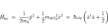 |
(A.33) |
( is identical with
 of equations
(2.29a) and (2.31)
before scaling)
one obtains for the time evolution of
after
time
of equations
(2.29a) and (2.31)
before scaling)
one obtains for the time evolution of
after
time  :
:
 |
(A.34) |
that is, again a
(different)
coherent state, except for a phase factor.
Therefore the uncertainties
 ,
,
 are
conserved, which is just the expected behaviour for a classical
particle.A.9Further information about the time evolution of coherent states may be
found in [Ger92].
are
conserved, which is just the expected behaviour for a classical
particle.A.9Further information about the time evolution of coherent states may be
found in [Ger92].
The equations
(A.39-A.43)
also show that the state
 of equation (A.29)
in fact is a coherent state up to a phase factor,
of equation (A.29)
in fact is a coherent state up to a phase factor,
![\begin{displaymath}
\left< x \left\vert \alpha \right> \right.
\; = \; \sqrt[4]...
...rt x',p' \right> \right. e^{-i\textstyle \frac{x'p'}{2\hbar}},
\end{displaymath}](img1381.png) |
(A.34) |
and
with equation (A.30) one has for the antinormal-ordered
distribution function:
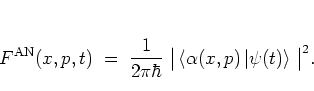 |
(A.35) |
For this reason the antinormal-ordered distribution function is often
called the coherent state representation of the state
 (see e.g. [ABB96]).
It is
interesting to note that the set of coherent
states
is
overcomplete:
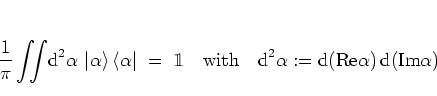 |
(A.36) |
-- in contrast, for instance, to the set
 of eigenstates of the harmonic
oscillator, which is ``only'' complete. Overcompleteness of
of eigenstates of the harmonic
oscillator, which is ``only'' complete. Overcompleteness of
 is indicated by the factor
 in equation (A.52).
Overcompleteness
of
guarantees that every state
in equation (A.52).
Overcompleteness
of
guarantees that every state
 can
be expanded into a superposition of coherent states; but due to the
nonorthogonality of these states as expressed by equation
(A.36) this expansion is not unique, in general.A.10
can
be expanded into a superposition of coherent states; but due to the
nonorthogonality of these states as expressed by equation
(A.36) this expansion is not unique, in general.A.10
Using the overcompleteness property (A.52) of the
coherent states and the expression (A.51) for
 it is easy to show that the antinormal-ordered distribution
is normalized in the sense of
it is easy to show that the antinormal-ordered distribution
is normalized in the sense of
 |
(A.37) |
For more information on coherent states I refer the reader to the
specialist literature: the monograph [KS85]
remains
the standard work
in this field;
some more recent studies are
for example [WK93,KWZ94,ZK94],
where among other questions the problem of coherent states in
finite-dimensional HILBERT spaces is addressed.
Finally, in [Nie97a] NIETO presents an interesting
overview of the historic development of the theory of coherent states
as well as of the squeezed states which I
discuss in the following
subsection.
Footnotes
- ...
dynamics.A.8
- But note that SCHRÖDINGER's generalizing
interpretation in [Sch26]
of this
feature of the
harmonic oscillator
is erroneous.
See [Str01b] for
some background material on this issue.
- ...
particle.A.9
-
Moreover, for the present case of the harmonic oscillator
EHRENFEST's theorem
allows to conclude
that the dynamics of the mean values
of the position and momentum operators coincide with the classical
dynamics of the
observables
 and
and  , namely a harmonic
oscillation bounded by turning points which
are determined by the energy
, namely a harmonic
oscillation bounded by turning points which
are determined by the energy
 :
:
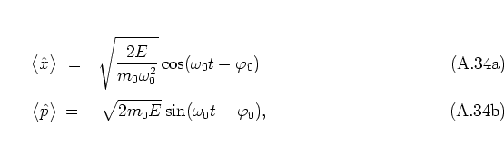
with the phase shift
 .
.
- ... general.A.10
-
By imposing certain additional conditions on the expansion
coefficients
it is still possible to achieve a unique expansion
in terms of
coherent states. More on this GLAUBER expansion can be found
in [Per93].
Next: Squeezed States
Up: Minimum Uncertainty States and
Previous: Minimum Uncertainty States and
Contents
Martin Engel 2004-01-01