Next: Minimum Uncertainty States and
Up: Quantum Phase Space Distribution
Previous: Definition of Quantum Phase
Contents
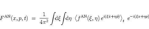
In the same way in which the
kernel
 determines the
association between operators and scalars, it also defines an
operator ordering [Meh77,AM77].
In this context
an expansion (A.7) of an
operator is called ordered if it
is written as
a superposition of terms
that
are of
the form
determines the
association between operators and scalars, it also defines an
operator ordering [Meh77,AM77].
In this context
an expansion (A.7) of an
operator is called ordered if it
is written as
a superposition of terms
that
are of
the form
 .
The essential point of this definition is that the multiplication of the
exponential
.
The essential point of this definition is that the multiplication of the
exponential
 with the kernel function
yields a
characteristic composition of exponential operators, the explicit form of
which depends on the particular choice of
with the kernel function
yields a
characteristic composition of exponential operators, the explicit form of
which depends on the particular choice of  .
.
The implications of this definition become clearer
when some specific examples are considered:
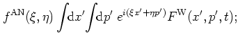
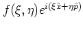
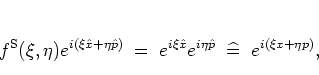
- For the kernel function
 |
(A.10) |
one obtains from equation (A.13),
integrating over  and
and  and substituting
 ,
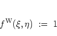
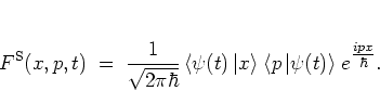
the WIGNER distribution function [Wig32]:
,
the WIGNER distribution function [Wig32]:
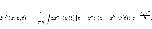 |
(A.11) |
It corresponds to the WEYL ordering of operators
[Wey31,DGS72],
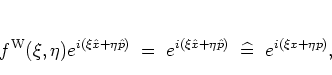 |
(A.12) |
and by equations (A.7, A.8)
gives rise to the WEYL transform
of the
operator  :
:
 |
(A.13) |
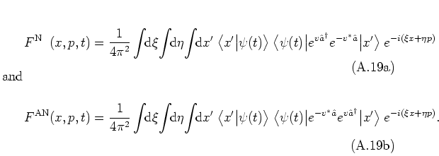
The last two terms of
expression (A.16) indicate
the association of operators and scalars that is defined by
 ,
as discussed in section A.1.
,
as discussed in section A.1.
Using the WIGNER distribution function, the overlap of two states
 and
and
 described by the
WIGNER functions
described by the
WIGNER functions  and
and  can be computed as the overlap of the
corresponding
WIGNER functions in phase space:
can be computed as the overlap of the
corresponding
WIGNER functions in phase space:
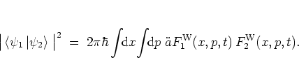 |
(A.14) |
Besides the HUSIMI distribution function (which is introduced in section
A.3 below), the WIGNER function is the most commonly used
quantum phase space distribution function.
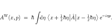
- The kernel function
 |
(A.15) |
defines the standard ordering of operators; it is characterized by
all  -dependent terms preceding the
  -dependent terms,
 |
(A.16) |
which leads to the standard-ordered distribution
functionA.4:
 |
(A.17) |
Essentially,
 is
the product of the position and momentum representations of the state
is
the product of the position and momentum representations of the state
 .
.
- Setting
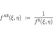 |
(A.18) |
and thus
having all -dependent terms precede the -dependent terms,
one gets the antistandard-ordered distribution function (also
known as the
KIRKWOOD distribution function [Kir33] or
RIHACZEK distribution function [Rih68]):
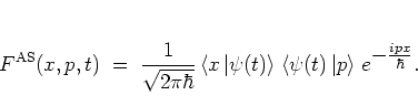 |
(A.19) |
It is obtained from its standard-ordered counterpart
by complex conjugation.
- For systems that can be described as a harmonic oscillator with mass
 and frequency
  -- in this appendix no scaling as in
section 2.1
is employed, such that
the parameters and are retained in the formulae -- or as
an ensemble of harmonic oscillators, the normal-ordered and the antinormal-ordered distribution
functions
-- in this appendix no scaling as in
section 2.1
is employed, such that
the parameters and are retained in the formulae -- or as
an ensemble of harmonic oscillators, the normal-ordered and the antinormal-ordered distribution
functions
 and
and
 are
useful.A.5They are defined by requiring operators to be (anti-)
standard-ordered not with respect to , , but with respect to the
ladder operators, i.e. with respect to the creation operator
are
useful.A.5They are defined by requiring operators to be (anti-)
standard-ordered not with respect to , , but with respect to the
ladder operators, i.e. with respect to the creation operator
 and the annihilation operator
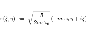
  , where is given by
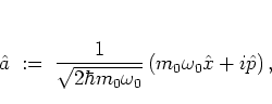 |
(A.20) |
as usual. (Equation (2.30) is obtained from this
definition in the case of
the scaling
(1.15, 2.4),
i.e. by formally setting
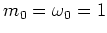 .)
.)
This (anti-) standard ordering of operators is
achieved by using the kernels
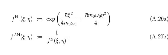
as can easily be
confirmed by direct computation:A.6
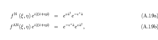
where the complex parameter  is defined as
 |
(A.19) |
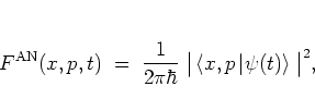
The corresponding distribution functions are
The normal-ordered distribution
 is also called
GLAUBER-SUDARSHAN distribution function or
is also called
GLAUBER-SUDARSHAN distribution function or
 -function [Gla63b,Gla65,Sud63], while
the antinormal-ordered distribution
-function [Gla63b,Gla65,Sud63], while
the antinormal-ordered distribution
 is sometimes referred to as the
 -function [Gla65].
Defining
 as a Gaussian wave packet centered at
 in phase space,A.7
![\begin{displaymath}
\left< x \left\vert x',p' \right> \right. \; = \; \sqrt[4]{\...
...0\omega_0}{2\hbar}(x-x')^2}
e^{\textstyle \frac{ip'x}{\hbar}}
\end{displaymath}](img1333.png) |
(A.19) |
with
 , the antinormal-ordered distribution function
can be written in a particularly concise way:
, the antinormal-ordered distribution function
can be written in a particularly concise way:
 |
(A.20) |
as is easily verified by substituting formula (A.29) into
equation (A.30) and comparing the result with the definition
(A.13) for
 .
.
Therefore,
is essentially obtained by
computing the convolution of the state
with a Gaussian
in position space. The physical meaning of this convolution
becomes
clearer in section A.5.
From equation (A.30) it is also clear that is
non-negative; this
is of importance
for the interpretation of as a (quasi-) probability
distribution function in section A.5.
in the
form of equation (A.30)
finds
its main application in
the discussion of the HUSIMI distribution function in section
A.3.
Since there are
infinitely
many different functions that
can be chosen as kernel functions, there exist equally many different
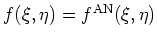
distribution functions  . The important point
is that all these different
. The important point
is that all these different  are equivalent: each of them contains
the same information about the state
, and each can
be used to compute the expectation values (A.9a) of any
operator
are equivalent: each of them contains
the same information about the state
, and each can
be used to compute the expectation values (A.9a) of any
operator
 that is expanded as in equation (A.7).
The connection between the WIGNER distribution function and the
antinormal-ordered distribution function is an important example:
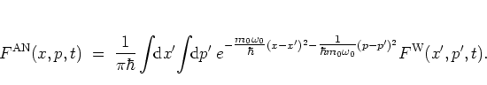 |
(A.21) |
This unveils the antinormal-ordered distribution function as the
convolution of the WIGNER function with a Gaussian in
phase space; I
discuss this fact in some more detail in section
A.5.
Formula (A.31) may be proved in the following way:
using similar arguments as those
leading to equation (A.13),
with the definition (A.6)
I first rewrite
as
 |
(A.22) |
and obtain for the expectation value in the integrand:
equation (A.31) then follows by integration over and
 .
.
Other conversion formulae between arbitrary different distribution
functions
 and
and
 with
with  can be obtained by similar computations.
Some formulae of this type are listed in [Lee95].
can be obtained by similar computations.
Some formulae of this type are listed in [Lee95].
Footnotes
- ...
functionA.4
-
This slightly inaccurate naming convention is
common practice. In order to avoid misunderstandings I want to
stress here that in the narrow sense it is only operators that
are (or are not) standard-ordered.
For distribution functions (standard) ordering is
not defined at all.
Therefore, the standard-ordered distribution is not
standard-ordered. Similar statements hold for all the other
orderings of operators and their associated distribution functions.
- ...
useful.A.5
-
Typical applications may be found in quantum optics;
see [Vou94,KH95b] for some examples.
Another field where
 and
and  are utilized frequently
is the modelling of a heat bath by an ensemble of harmonic oscillators
[Coh94,HB95,HB96].
Cf. also the monographs by Louisell [Lou64,Lou73]
and Dineykhan et al. [DEGN95].
are utilized frequently
is the modelling of a heat bath by an ensemble of harmonic oscillators
[Coh94,HB95,HB96].
Cf. also the monographs by Louisell [Lou64,Lou73]
and Dineykhan et al. [DEGN95].
- ... computation:A.6
-
For more information on (anti-) normal ordering of operators see
[DEGN95].
- ... space,A.7
-
A Gaussian wave packet like
 is often referred to
as a coherent state. Such a state is characterized by
is often referred to
as a coherent state. Such a state is characterized by
 ,
,
 ,
,
 and
and
 ,
such that
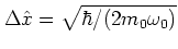
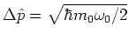
is a state with minimum uncertainty product:
,
such that
is a state with minimum uncertainty product:
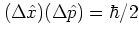 .
In section A.3 I discuss coherent states from a more
general point of view and an important generalization of this concept.
.
In section A.3 I discuss coherent states from a more
general point of view and an important generalization of this concept.
Next: Minimum Uncertainty States and
Up: Quantum Phase Space Distribution
Previous: Definition of Quantum Phase
Contents
Martin Engel 2004-01-01