One possible motivation for introducing quantum distribution functions is their utility for the comparison of classical and quantum mechanics, as mentioned above. In addition to this there is another, equally important motivation for studying these functions: they can be used to compute expectation values in a comparatively simple way, where the computational simplification is mainly due to the fact that the corresponding formulae depend on scalars only, as opposed to conventional expressions of quantum expectation values which typically involve operators.
Consider a classical observable ![]() that depends on the position and
momentum variables
that depends on the position and
momentum variables ![]() and
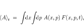
and ![]() . The expectation value of
. The expectation value of ![]() can be
computed as
can be
computed as
Rather than discussing
a general
quantum
observable
![]() , with the
position and the momentum operators
, with the
position and the momentum operators ![]() and
and ![]() , I begin by
considering a particular operator instead, namely
, I begin by
considering a particular operator instead, namely
![]() ,
with constants
,
with constants
![]() .
Exponentials of this type are used below in the FOURIER expansion
(A.7) to construct any other operator.
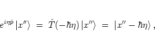
In order to obtain an expression analogous to equation (A.1)
the operator
.
Exponentials of this type are used below in the FOURIER expansion
(A.7) to construct any other operator.
In order to obtain an expression analogous to equation (A.1)
the operator
![]() somehow has to be substituted by a
corresponding scalar expression. For example one could set
somehow has to be substituted by a
corresponding scalar expression. For example one could set
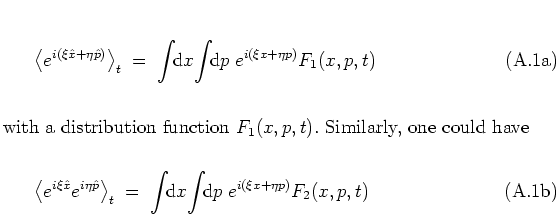
as well, with
another
distribution function ![]() .
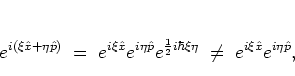
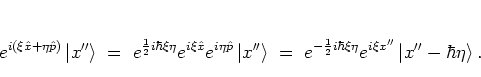
But due to the fact that
.
But due to the fact that ![]() and
and ![]() do not commute one has
do not commute one has
 |
(A.1) |
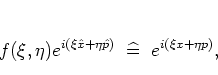
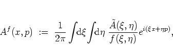
In order to avoid this ambiguity one first chooses a complex-valued
kernel function ![]() ; then the scalar
; then the scalar
![]() is defined to be associated with the operator
is defined to be associated with the operator
![]() exclusively,
exclusively,
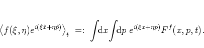
The
quantization rule
(A.5) not only defines how to
associate exponential operators with scalars, but is much more general,
as it can be applied to each term of the FOURIER expansion of any
operator ![]() ,
,
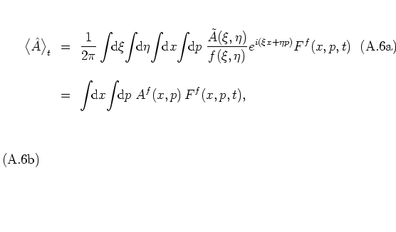
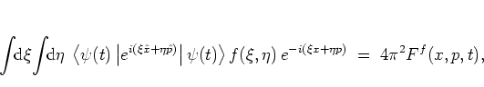
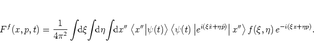
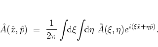
An explicit expression for the distribution function
![]() can be obtained from the implicit definition (A.6) by
FOURIER transformation. For a system in the state
can be obtained from the implicit definition (A.6) by
FOURIER transformation. For a system in the state
![]() at
time
at
time ![]() , the expectation values are given by
, the expectation values are given by
![]() , and one gets
, and one gets
Note that
the kernel function
can
also
be chosen,
more generally,
as a functional
of the quantum state
![]() of the system
itself:
of the system
itself:
![]() .
COHEN
gives an example for such a kernel function
.
COHEN
gives an example for such a kernel function
![]() that, despite being quite
complicated, leads to the very simple
COHEN distribution function
that, despite being quite
complicated, leads to the very simple
COHEN distribution function
![]() that nicely combines the position and momentum representations of
that nicely combines the position and momentum representations of
![]() in an intuitive way
[Coh66].
However,
since choosing a
in an intuitive way
[Coh66].
However,
since choosing a ![]() -dependent
-dependent ![]() has a number of unfavourable consequences -- for
example, equation (A.8) indicates that
in this case
the function
has a number of unfavourable consequences -- for
example, equation (A.8) indicates that
in this case
the function
![]() associated with the operator
associated with the operator ![]() becomes
becomes ![]() -dependent, too -- I
do not further discuss kernels that
are functionals of
-dependent, too -- I
do not further discuss kernels that
are functionals of
![]() .
.
![\begin{displaymath}
\hspace*{-0.4cm}
\fbox{$ \displaystyle
\begin{array}{rcl...
...}.
\rule[-0.5cm]{0.0cm}{1.0cm}\hspace*{0.1cm}
\end{array} $}
\end{displaymath}](img1291.png)
![\begin{displaymath}
e^{\hat{A}}e^{\hat{B}}\; = \; e^{{\hat{A}}+{\hat{B}}}e^{\frac{1}{2}[{\hat{A}},{\hat{B}}]}
\end{displaymath}](img1263.png)