With the results of the previous subsections it is now but a small step to
the definition of the HUSIMI distribution function. Replacing in
equation (A.27) the frequency ![]() of the harmonic oscillator
with an arbitrary
of the harmonic oscillator
with an arbitrary
![]() (the interrelation of which
with
squeezed states is illustrated by equation
(A.69)),
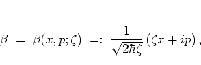
a complex number
(the interrelation of which
with
squeezed states is illustrated by equation
(A.69)),
a complex number ![]() is defined:
is defined:
At this point the discussion has moved quite a distance away from the
original harmonic oscillator: direct contact with it was lost when the
generalized ladder operators ![]() ,
, ![]() were introduced in
subsection A.3.2 in order to replace the original
were introduced in
subsection A.3.2 in order to replace the original
![]() ,
,
![]() in an ad hoc fashion; the oscillator frequency
in an ad hoc fashion; the oscillator frequency
![]() has been substituted by the abstract quantity
has been substituted by the abstract quantity ![]() , and the
only remaining original parameter of the oscillator is its mass
, and the
only remaining original parameter of the oscillator is its mass ![]() .
Therefore it
is
reasonable to leave the original oscillator terminology
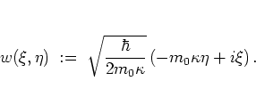
behind altogether and define the new real parameter
.
Therefore it
is
reasonable to leave the original oscillator terminology
behind altogether and define the new real parameter
 |
(A.45) |
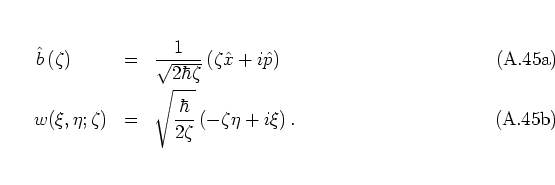
With these ![]() and
and ![]() replacing
replacing ![]() and
and ![]() in equation (A.28b),
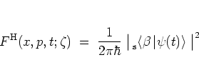
one finally arrives at the ``celebrated''
HUSIMI distribution function [Hus40]:
in equation (A.28b),
one finally arrives at the ``celebrated''
HUSIMI distribution function [Hus40]:
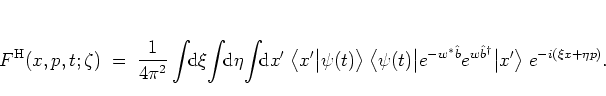
For this calculation, which is an application of the formalism outlined
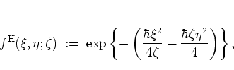
in section A.1, the kernel function
![]() defining
defining
![]() is needed.
It is easy to see that this kernel function is
is needed.
It is easy to see that this kernel function is
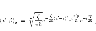
For the practical
evaluation
of the formula (A.74)
for the HUSIMI function normally the
position
representation of the
squeezed state
![]() ,
,
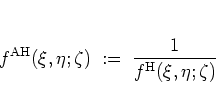
In line with the formalism of section A.1, as a byproduct
the definition (A.76)
in a natural way leads
to the introduction of yet another
distribution function which is the counterpart of the HUSIMI function in
the same way
in which
the antinormal-ordered distribution function is the
counterpart of the normal-ordered
distribution:
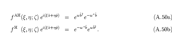
with the definition
 |
(A.50) |
Finally, it remains to specify the operator orderings themselves that are
associated with these distribution functions. Not surprisingly it turns
out that the anti-HUSIMI and the HUSIMI distribution functions
correspond to standard ordering and anti-standard ordering with respect to
the generalized ladder operators ![]() ,
, ![]() , respectively:
, respectively:
In section A.5 I discuss in some more detail the
significance of the parameter ![]() and how this parameter can be used
in the course of the analysis of a physical state
and how this parameter can be used
in the course of the analysis of a physical state
![]() .
.