One of the defining properties of classical periodic stochastic webs is
their translational invariance.
Therefore it is natural to look for a similar property in the quantum
realm.
To this end, the commutation properties of the
FLOQUET operator ![]() , as given by
equations (2.28, 2.32a, 2.35a),
with respect to
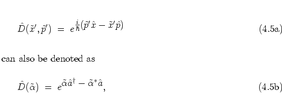
the displacement operator
, as given by
equations (2.28, 2.32a, 2.35a),
with respect to
the displacement operator
![]() (equations (4.1))
need to be considered.
(equations (4.1))
need to be considered.
For
the first contribution to ![]() ,
the kick propagator
,
the kick propagator
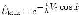 ,
,
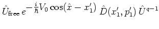
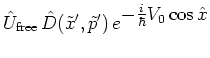
Next
I consider the propagator
![]() which describes
the free harmonic oscillator dynamics.
At this stage of the
present
discussion,
which describes
the free harmonic oscillator dynamics.
At this stage of the
present
discussion, ![]() is not yet restricted to one of the
resonance values specified in equation (1.23), but
can take on any value.
Since
is not yet restricted to one of the
resonance values specified in equation (1.23), but
can take on any value.
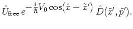
Since
![]() brings about
clockwise rotation in
phase space through the angle
brings about
clockwise rotation in
phase space through the angle ![]() ,
corresponding to the free part
,
corresponding to the free part
![]() of the
classical web map (1.20c),
the operators
of the
classical web map (1.20c),
the operators
![]() and
and
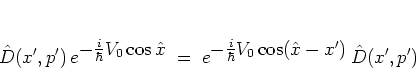
![]() can be interchanged by introducing
a new set
can be interchanged by introducing
a new set
![]() of parameters which is obtained from
of parameters which is obtained from
![]() by anti-clockwise rotation through
by anti-clockwise rotation through
![]() :
:
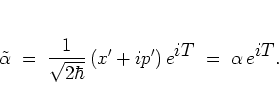
with the real parameters
![\begin{subequations}
\begin{eqnarray}
\tilde{x}' & = & x'\cos T - p'\sin T \\ [0.3cm]
\tilde{p}' & = & x'\sin T + p'\cos T
\end{eqnarray}\end{subequations}](img730.png)
-- cf. equation (1.20c).
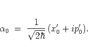
Using the definition
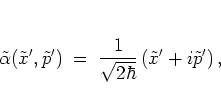 |
(4.5) |
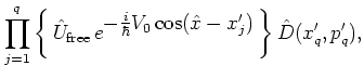
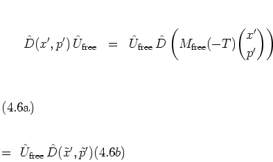
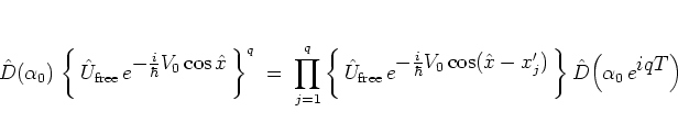
Combination of equations (4.10) and (4.11b) with the
splitting (2.28) then gives
 |
|||
 |
(4.6) |
![\begin{subequations}
\begin{eqnarray}
x_j' & = & x_0'\cos jT - p_0'\sin jT \\ [-...
...\ [-0.1cm]
p_j' & = & x_0'\sin jT + p_0'\cos jT
\end{eqnarray}\end{subequations}](img743.png)
 |
(4.8) |
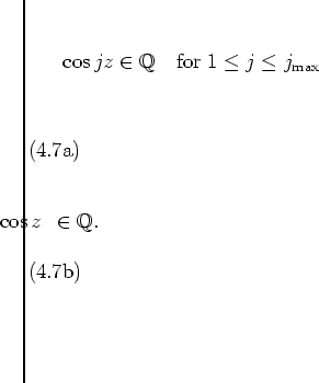
Concluding from equation (4.19), the
operators
![]() and
and ![]() commute
if and only if
there are integers
commute
if and only if
there are integers
![]() such that
such that
![\begin{subequations}
\begin{eqnarray}
qT & = & 2\pi l
\\ [0.3cm]
x_j' & = & 2\pi k_j \qquad \mbox{for} \quad 1\leq j\leq q .
\end{eqnarray}\end{subequations}](img750.png)
These conditions need to be analyzed further in order to understand
the consequences for the quantum phase portrait, but some consequences
can be read off from equations (4.21) directly.
Equation (4.21a) imposes a restriction on
the rotational part
![]() of the FLOQUET operator
and thus leads to rotational symmetries.
For general values of
of the FLOQUET operator
and thus leads to rotational symmetries.
For general values of ![]() , equation (4.21a)
is identical with the general classical resonance condition
(1.22).
For
, equation (4.21a)
is identical with the general classical resonance condition
(1.22).
For ![]() it restricts the values of
it restricts the values of ![]() to
to
In the context of equation (4.19),
a lucid interpretation of the resonance condition
(1.23/4.22) can be given:
it refers to symmetries that come about after the ![]() successive
applications of
successive
applications of
![]() in equation (4.19) have
accounted for exactly one full rotation in phase space.
For general values of
in equation (4.19) have
accounted for exactly one full rotation in phase space.
For general values of ![]() ,
,
![]() belongs to
the more general category of resonances as defined
by equation (1.22),
corresponding to
belongs to
the more general category of resonances as defined
by equation (1.22),
corresponding to ![]() rotations in phase space after
rotations in phase space after ![]() applications of
applications of
![]() .
Below I show
that it suffices to consider the simplest case
.
Below I show
that it suffices to consider the simplest case ![]() in order to discuss and explain the symmetries of the quantum stochastic
webs that have been observed in the previous two sections.
in order to discuss and explain the symmetries of the quantum stochastic
webs that have been observed in the previous two sections.
Combination of equation (4.21a) with the
definition (4.18) for ![]() shows that the resonance
condition
implies
shows that the resonance
condition
implies
![\begin{subequations}
\begin{eqnarray}
x_q' & = & x_0'
\\ [0.3cm]
p_q' & = & p_0' ,
\end{eqnarray}\end{subequations}](img754.png)
which is another way of expressing that
a full rotation in phase space is obtained after not more than ![]() iterations of
iterations of ![]() .
.
Equation (4.21b) determines the allowed
translations and therefore concerns the translational symmetries of
the phase portrait.
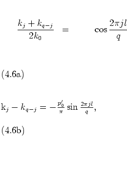
Substituting equation (4.21b) into the
definitions (4.18),
is obtained;
here, ![]() is used,
which is consistent with equation (4.23a).
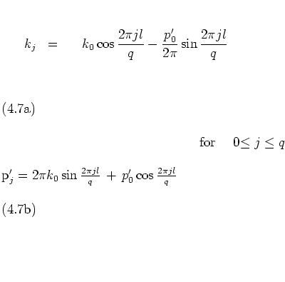
Equation (4.24a) can be rewritten in the form
is used,
which is consistent with equation (4.23a).
Equation (4.24a) can be rewritten in the form
which holds for
![]() and
and
![]() with
with
 |
(4.7) |
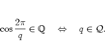
Note that
-- with any
![]() , and in fact with any
, and in fact with any
![]() --
the following
two
assertions
are equivalent:
--
the following
two
assertions
are equivalent:
This is a useful observation, since
it allows to discuss the
rationality
of
![]() for all
for all
![]() by considering just the case of
by considering just the case of ![]() .
The equivalence of (4.28a) and (4.28b)
can be
shown
in the following way.
Clearly, (4.28b) is implied by (4.28a)
with
.
The equivalence of (4.28a) and (4.28b)
can be
shown
in the following way.
Clearly, (4.28b) is implied by (4.28a)
with ![]() .
Conversely, assuming that
.
Conversely, assuming that ![]() is rational, the same is true for
is rational, the same is true for
![]() .
Rationality of
.
Rationality of ![]() for all
for all ![]() then follows by induction
using
then follows by induction
using
 |
(4.7) |
Finally, for general values of
![]() one has the
result that
one has the
result that
For simplicity, from here on I consider
the case of ![]() only.
Higher order symmetries that are associated with
only.
Higher order symmetries that are associated with
![]() are thus excluded from the following considerations. On the other hand,
the choice
are thus excluded from the following considerations. On the other hand,
the choice ![]() is sufficient to discuss and explain the symmetries of
the quantum stochastic webs
that have been
observed in the previous two subsections.
is sufficient to discuss and explain the symmetries of
the quantum stochastic webs
that have been
observed in the previous two subsections.
Combining the above arguments
(4.25-4.30),
it is
now
shown that if ![]() satisfies the classical
resonance condition
(1.23) with
satisfies the classical
resonance condition
(1.23) with
![]() ,
then integers
,
then integers
![]() can in fact be
found
which satisfy equation (4.25a),
and therefore
equation (4.24a) as well,
provided the
can in fact be
found
which satisfy equation (4.25a),
and therefore
equation (4.24a) as well,
provided the ![]() are chosen suitably.
This being granted, the result
are chosen suitably.
This being granted, the result
![\begin{displaymath}
\left[ \hat{D}(x_0',p_0'), \, {\hat{U}}^q \right] \; = \; 0
\end{displaymath}](img779.png) |
(4.9) |
In this way
the classical resonance condition
with
![]() is proven to be a necessary condition for the existence of
periodic quantum stochastic webs;
in this sense it plays the same role both in classical and quantum
mechanics.
This observation is supported by the fact that the results described
above are obtained irrespective of the values of
is proven to be a necessary condition for the existence of
periodic quantum stochastic webs;
in this sense it plays the same role both in classical and quantum
mechanics.
This observation is supported by the fact that the results described
above are obtained irrespective of the values of ![]() and
and ![]() .
As in the classical case, the
overall
structure of the stochastic web is
entirely and solely determined by the parameter
.
As in the classical case, the
overall
structure of the stochastic web is
entirely and solely determined by the parameter ![]() .
.
In order to check that the
![]() determined in accordance with equation
(4.25a) also satisfy (4.24a)
it remains to check that equation (4.25b) is
obeyed, too.
In particular, it must be confirmed that the
determined in accordance with equation
(4.25a) also satisfy (4.24a)
it remains to check that equation (4.25b) is
obeyed, too.
In particular, it must be confirmed that the
![]() determined by
equation (4.24a) are indeed integers, as required by equation
(4.21b).
This cannot be discussed in general terms, but needs to
be checked for each individual
determined by
equation (4.24a) are indeed integers, as required by equation
(4.21b).
This cannot be discussed in general terms, but needs to
be checked for each individual
![]() .
.
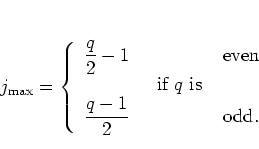
Evaluating equation (4.24a) it turns out
-- not surprisingly --
that the cases of ![]() , belonging to
, belonging to ![]() but not
to
but not
to
![]() , are
in a characteristic way
different from the cases of
, are
in a characteristic way
different from the cases of
![]() belonging to
belonging to
![]() .
In the following equations, both
.
In the following equations, both
![]() and
and ![]() are integers that can be chosen as desired.
are integers that can be chosen as desired.
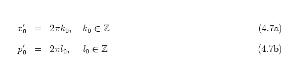
The symmetric quantum phase space structures obtained for
![]() and
and ![]() are identical. The restrictions discussed above imply that the
parameters
are identical. The restrictions discussed above imply that the
parameters ![]() describing the translational symmetries
have to be chosen according to
describing the translational symmetries
have to be chosen according to
![\begin{subequations}
\begin{eqnarray}
x_0' & = & 2\pi k_0, \quad k_0\in\mathbb{Z}\\ [0.3cm]
p_0' & \in & \mathbb{R}.
\end{eqnarray} \end{subequations}](img785.png)
The phase portrait is periodic in ![]() -direction with period
-direction with period ![]() ;
translations by
;
translations by ![]() in
in ![]() -direction are admissible with any
-direction are admissible with any
![]() .
This is exactly the symmetry pattern visible in the contour
plot 1.9 of the classical time averaged
Hamiltonians
.
This is exactly the symmetry pattern visible in the contour
plot 1.9 of the classical time averaged
Hamiltonians
![]() ,
,
![]() .
And while it is not confirmed
-- due to the limited number of iterations --
by the quantum phase portraits
C.38-C.40
for
.
And while it is not confirmed
-- due to the limited number of iterations --
by the quantum phase portraits
C.38-C.40
for ![]() (see section C.3 of the appendix),
these figures at least do not stand in contradiction to the
symmetries described here.
(see section C.3 of the appendix),
these figures at least do not stand in contradiction to the
symmetries described here.
For these values of ![]() , translational invariance is obtained with
respect to the translations given by
, translational invariance is obtained with
respect to the translations given by
![\begin{subequations}
\begin{eqnarray}
x_0' & = & 2\pi k_0 \\ [-0.15cm]
& & \hs...
... \frac{2\pi}{\sqrt{3}}\left(k_0+2l_0\right) ,
\end{eqnarray} \end{subequations}](img790.png)
in agreement with both the skeleton of the classical stochastic webs
displayed in figure 1.10a and the quantum
phase portraits
4.4-4.6
and
C.18-C.37
(in the appendix)
for ![]() and
and ![]() .
.
In this case, the translations
are obtained, reproducing the classical square grid of figure
1.10b and of the quantum stochastic webs for ![]() in
figures
4.2,
4.3,
4.7
and
C.1-C.17.
in
figures
4.2,
4.3,
4.7
and
C.1-C.17.
In this way, the symmetries of the quantum stochastic webs that have been
obtained in
subsection 4.1.1
using
numerical means are explained
analytically by exploiting the translation invariance of the FLOQUET operator. This explanation
of the infinitely extended eigenstates of the system
works for all
![]() and for all values of
and for all values of
![]() and
and ![]() .
.
Note that this analytical explanation of the quantum skeletons nicely
parallels the analytical explanation of the skeletons of classical
stochastic webs (see subsection 1.2.2)
in the following sense:
the rotational and translational symmetries of the quantum webs arise from
the combination of
![]() and
and
![]() .
None of these operators alone gives rise to the symmetries of the webs.
The same is true for
.
None of these operators alone gives rise to the symmetries of the webs.
The same is true for
![]() and
and
![]() with respect to the classical webs
-- cf. the footnote on page
with respect to the classical webs
-- cf. the footnote on page ![[*]](crossref.png) .
In summary, both the classical and quantum stochastic webs are the
result of the combination of both indispensable contributions
.
In summary, both the classical and quantum stochastic webs are the
result of the combination of both indispensable contributions
![]() and
and
![]() to the Hamiltonian.
In particular, the symmetries of the quantum webs do not reflect
any symmetries of the elements of the basis
to the Hamiltonian.
In particular, the symmetries of the quantum webs do not reflect
any symmetries of the elements of the basis
![]() used for expanding the quantum states in the web.
used for expanding the quantum states in the web.