The Classical Limit

It is instructive to use the quantum mechanical system introduced in the previous section to rederive the classical POINCARÉ map (1.21). This is most conveniently done in the HEISENBERG picture, rather than in the SCHRÖDINGER picture that has been used in section 2.1 to formulate the quantum map. In the present section, and only here, I use the indices ${}_{\mbox{\tiny H}}$ and ${}_{\mbox{\tiny S}}$ in order to distinguish between HEISENBERG and SCHRÖDINGER operators. (All operators used elsewhere without explicit reference to a particular picture are SCHRÖDINGER operators.)

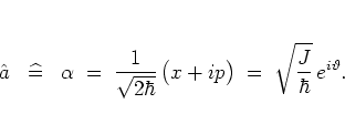
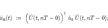
Using the time evolution operator ${\hat{U}}(t',t)$, the time-dependent annihilation operator ${\hat{a}_{\mbox{\tiny H}}}(t)$ can be defined as

$${\hat{a}_{\mbox{\tiny H}}}(t) \; := \; \left( {\hat{U}}(t,nT... ...ht)^\dagger \, {\hat{a}_{\mbox{\tiny S}}}\; {\hat{U}}(t,nT-0);$$ (2.42)

the time-independent annihilation operator ${\hat{a}_{\mbox{\tiny S}}}$ has been defined in equation (2.30a), and the initial condition

$${\hat{a}_{\mbox{\tiny H}}}(nT-0) \; := \; {\hat{a}_{\mbox{\tiny S}}}$$ (2.43)

immediately before the $n$-th kick has been chosen. This choice facilitates the comparison with the classical POINCARÉ map further below.

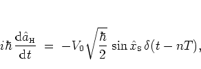
The dynamics of ${\hat{a}_{\mbox{\tiny H}}}(t)$ is governed by the HEISENBERG equation of motion [Mes91],

$$i\hbar \, \frac{{\mbox{d}}{\hat{a}_{\mbox{\tiny H}}}}{{\mbo... ...t[{\hat{a}_{\mbox{\tiny H}}},{\hat{H}_{\mbox{\tiny H}}}\right]$$ (2.44)

$[\cdot,\cdot]$ being the usual commutator. For the kick dynamics at the $n$-th kick I have

$$i\hbar \, \frac{{\mbox{d}}{\hat{a}_{\mbox{\tiny H}}}}{{\mbo... ...bar}V_0\cos{\hat{x}_{\mbox{\tiny S}}}} \right] \delta(t-nT),$$ (2.45)

where I have discarded the time-independent part of the Hamiltonian ${\hat{H}_{\mbox{\tiny S}}}$ (2.5) and used the expression (2.35a) for ${\hat{U}}_{\mbox{\scriptsize kick}}= {\hat{U}}(nT+0,nT-0)$. Equation (2.55) and the following expressions up to (2.59) hold for $t\in[nT-\varepsilon,nT+\varepsilon]$ in the limit of $\varepsilon\to 0$ only. Using equation (2.52) and well-known commutator algebra, the commutator on the right hand side can be written as

$$e^{ \textstyle \frac{i}{\hbar}V_0\cos{\hat{x}_{\mbox{\tiny ... ...\textstyle -\frac{i}{\hbar}V_0\cos{\hat{x}_{\mbox{\tiny S}}}},$$

and by direct computation it is easily shown that

$$\left[ {\hat{a}_{\mbox{\tiny S}}},\cos{\hat{x}_{\mbox{\tiny... ...; = \; -\sqrt{\frac{\hbar}{2}} \sin{\hat{x}_{\mbox{\tiny S}}}.$$ (2.46)

Thus the HEISENBERG equation for the kick becomes

$$i\hbar \, \frac{{\mbox{d}}{\hat{a}_{\mbox{\tiny H}}}}{{\mbo... ...{\hbar}{2}} \, \sin{\hat{x}_{\mbox{\tiny S}}}\, \delta(t-nT),$$ (2.47)

which, with

$${\hat{x}_{\mbox{\tiny S}}}\; = \; {\hat{x}_{\mbox{\tiny H}}}(nT-0),$$ (2.48)

gives by integration over the kick

$${\hat{a}_{\mbox{\tiny H}}}(nT+0) \; = \; {\hat{a}_{\mbox{\t... ...{V_0}{\sqrt{2\hbar}} \, \sin{\hat{x}_{\mbox{\tiny H}}}(nT-0).$$ (2.49)

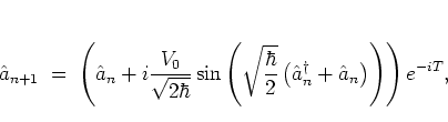
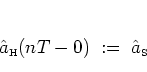
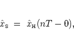
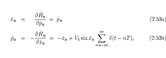
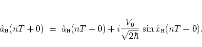
Solving the HEISENBERG equation between two consecutive kicks, i.e. for the unkicked harmonic oscillator, is somewhat easier. One has

$$i\hbar \, \frac{{\mbox{d}}{\hat{a}_{\mbox{\tiny H}}}}{{\mbo... ...{2} \right) \right] \; = \; \hbar {\hat{a}_{\mbox{\tiny H}}},$$ (2.50)

and therefore

$${\hat{a}_{\mbox{\tiny H}}}((n+1)T-0) \; = \; {\hat{a}_{\mbox{\tiny H}}}(nT+0) \, e^{-iT},$$ (2.51)

such that the complete quantum map in terms of the ladder operators is obtained as

$${\hat{a}}_{n+1} \; = \; \left( {\hat{a}}_n+i\frac{V_0}{\sqr... ...}_n^\dagger + {\hat{a}}_n \right) \right) \right) e^{-iT},$$ (2.52)

where the notation

$${\hat{a}}_n \; := \; {\hat{a}_{\mbox{\tiny H}}}(nT-0)$$ (2.53)

has been adopted for notational convenience; ${\hat{x}}_n$ and ${\hat{p}}_n$ (to be used below) are defined accordingly. By inversion of equations (2.30), substituting ${\hat{a}}_{n+1}$ and its Hermitian adjoint into the resulting expressions, and using equations (2.30) again, I finally get the quantum map for the position and momentum operators in the HEISENBERG picture:

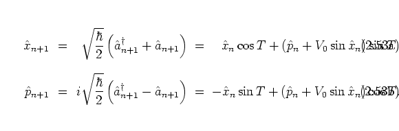
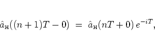
An equivalent way of deriving this form of the quantum map is to consider

$${\hat{H}_{\mbox{\tiny H}}}\; = \; \frac{1}{2}\left( {\hat{p... ...{\hat{x}_{\mbox{\tiny H}}}\sum_{n=-\infty}^\infty\delta(t-nT),$$ (2.53)

determine the canonical HEISENBERG equations of motion for ${\hat{x}_{\mbox{\tiny H}}}$ and ${\hat{p}_{\mbox{\tiny H}}}$,

and solve them in the same way as the classical equations of motion in subsection 1.1.3. In this way the discussion of the ladder operators as above is avoided; on the other hand the most condensed form (2.62) of the quantum map in the HEISENBERG picture is not obtained as a byproduct, but has to be derived afterwards, if desired.

Equations (2.62) and (2.64) contain exactly the same information as their SCHRÖDINGER picture counterpart (2.37), but especially equations (2.64) are better suited than the SCHRÖDINGER picture quantum map to make contact with the classical POINCARÉ map, as I show immediately.

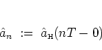
Substituting formally in the quantum map (2.64) the expectation values $\left< {\hat{x}} \right>_n$, $\left< {\hat{p}} \right>_n$ at time $nT$ for the operators ${\hat{x}}_n$, ${\hat{p}}_n$ results in just the equations (1.21) of the classical POINCARÉ map (where the expectation values take the places of the corresponding classical observables):

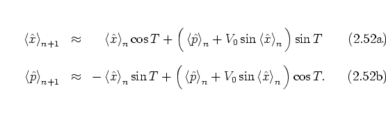
This clear formal analogy between the classical and quantum maps is one of the advantages of the HEISENBERG picture. Note that the transition from the quantum mechanically exact equations (2.64) to (2.67) is an approximation that cannot be justified in general terms. In fact it is generally a quite bad approximation the quality of which decreases with growing $\Delta {\hat{x}}$ and $\Delta {\hat{p}}$.

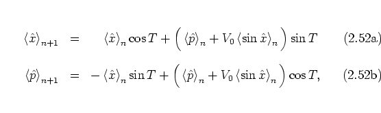
The same approximation may be accomplished by replacing the operators ${\hat{a}}$, ${\hat{a}}^\dagger$ in equation (2.62) by their associated $c$-numbers $\alpha$, $\alpha^*$ and taking into account the relationship of these with the classical observables $x$, $p$ (or equivalently with the action-angle variables $J$, $\vartheta$ of equation (1.35)):

$${\hat{a}}\;\;\; \widehat{=} \;\;\; \alpha \; = \; \frac{1}... ...g(x+ip\big) \; = \; \sqrt{\frac{J}{\hbar}} \, e^{i\vartheta}.$$ (2.52)

Decomposing the resulting expression into its real and imaginary parts, equations (2.67) are again obtained [Zas85].

The EHRENFEST equations of motion of the kicked harmonic oscillator, on the other hand, are obtained by taking the expectation values on both sides of equations (2.64) which gives the following, slightly different result:

the difference being marked by the fact that in general $\left< \sin{\hat{x}} \right>_n \neq \sin\left< {\hat{x}} \right>_n$. Equations (2.69) are quantum mechanically exact, in contrast to the approximative expressions (2.67). In the classical limit both the position and momentum distribution become $\delta$-peaked, as they describe a single classical point particle. In that limit $\left< \sin{\hat{x}} \right>_n$ and $\sin\left< {\hat{x}} \right>_n$ become equal and the EHRENFEST equations coincide with (2.67), thus becoming formally equivalent to their classical counterparts (1.21).

However, the way in which the limit of classical behaviour is reached is not obvious at all, among other reasons due to the fact that the expectation values are taken with respect to quantum states (solutions of the quantum map) about which not much is known a priori. In the following subsection I address this question from another point of view, by considering the explicit parameter dependence of the FLOQUET operator.