We now turn to the generic case where ![]() cannot be
decomposed into the direct sum of the kernel and range spaces of
cannot be
decomposed into the direct sum of the kernel and range spaces of ![]() .
As a trivial example for the way in which this problem arises,
consider a particle with a single degree of freedom (
.
As a trivial example for the way in which this problem arises,
consider a particle with a single degree of freedom (![]() ) which in
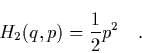
lowest order approximation is ``free'':
) which in
lowest order approximation is ``free'':
We
circumvent this problem by using Fredholm's alternative for ![]() :
:
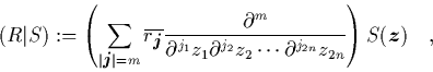
In accordance with (18) it is natural to define
a new normal form.
Let ![]() be a Hamiltonian of type (1a) with an arbitrary
quadratic contribution
be a Hamiltonian of type (1a) with an arbitrary
quadratic contribution ![]() . We say that
. We say that ![]() is
in generalized normal form up to order
is
in generalized normal form up to order ![]() if
if
Notice that (19) is not required to hold for ![]() --
in contrast to the corresponding definition (6) of the BGNF.
The reason being that in general it is impossible to normalize
--
in contrast to the corresponding definition (6) of the BGNF.
The reason being that in general it is impossible to normalize
![]() , since transforming
, since transforming ![]() implies changing
implies changing ![]() as well.
For generic
as well.
For generic ![]() one has to expect
one has to expect
![]() .
In Gustavson's case, however,
(6) is always true for
.
In Gustavson's case, however,
(6) is always true for ![]() , because the Poisson bracket
of
, because the Poisson bracket
of ![]() with itself vanishes.
with itself vanishes.
In order to
complete our definition of a normal form we have to specify the
explicit form of the scalar product.
For
![]() and
and
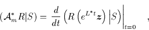
![]() we set [24,22]
we set [24,22]
We first write ![]() in yet another form. Linearizing Hamilton's
equations we obtain
the Hamiltonian matrix
in yet another form. Linearizing Hamilton's
equations we obtain
the Hamiltonian matrix
![]() , with the
, with the
![]() -dimensional symplectic matrix
-dimensional symplectic matrix
![$J = \left(\protect\begin{array}{@{}c@{\hspace*{0.1cm}}
c@{}}0&\mbox{\rm id}_n\\ [-0.1cm]-\mbox{\rm id}_n&0\protect\end{array}\right)$](img87.png) and the Hessian
and the Hessian
![]() .
Thus we have
.
Thus we have
In the form (22) ![]() can easily be used
for determining the splitting (18) of
can easily be used
for determining the splitting (18) of ![]() .
For the example (17) considered in the beginning of this section
we obtain
.
For the example (17) considered in the beginning of this section
we obtain
![]() and therefore
and therefore
![]() .
.
The method for transforming a given Hamiltonian into its generalized
normal form is exactly the same as the one described in the previous
section; one only has to replace (12b) by
| (15) |
Note that for a Hamiltonian of Gustavson's type (1) the two
definitions of normal form coincide, because in this case
![]() . So if
. So if ![]() is in BGNF (up to order
is in BGNF (up to order ![]() ) it is in
generalized normal form (up to order
) it is in
generalized normal form (up to order ![]() ), too.
The utility of the normal form will become evident in the next section.
), too.
The utility of the normal form will become evident in the next section.