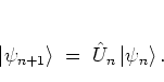
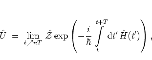
The natural quantum analogue of the classical map (1.21) is
obtained by considering the evolution of quantum states during one period
![]() of the excitation.
Therefore I define, in close analogy with (1.19), the
state
immediately before the
of the excitation.
Therefore I define, in close analogy with (1.19), the
state
immediately before the ![]() -th kick as
-th kick as
 |
(2.6) |
 |
(2.9) |
 |
(2.10) |
 |
(2.11) |
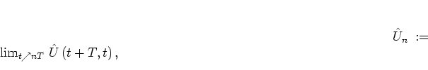
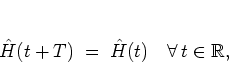
For a system with a time-periodic Hamiltonian
The
time-![]() -propagator
-propagator ![]() is also known as the FLOQUET operator of
the quantum system.
This naming convention is due to the fact that, using a
time-independent
orthonormal basis
is also known as the FLOQUET operator of
the quantum system.
This naming convention is due to the fact that, using a
time-independent
orthonormal basis
![]() of HILBERT space
for expanding
of HILBERT space
for expanding
![]() into
into
![]() , the time-dependent SCHRÖDINGER equation
(2.1) can be transformed into a system of ordinary
linear differential equations, the coefficients of which are
, the time-dependent SCHRÖDINGER equation
(2.1) can be transformed into a system of ordinary
linear differential equations, the coefficients of which are ![]() -periodic
because
-periodic
because
![]() exhibits the same periodicity.
For a finite basis this is the setting of the FLOQUET theorem which
asserts existence and uniqueness of the solutions and explicitly states
their functional dependence on
exhibits the same periodicity.
For a finite basis this is the setting of the FLOQUET theorem which
asserts existence and uniqueness of the solutions and explicitly states
their functional dependence on ![]() [Flo83,YS75]. In the present case the
FLOQUET theorem does not apply as the HILBERT space is
infinite-dimensional, but nevertheless the typical form of the FLOQUET solution and several other properties do carry over [Sal74].
Therefore, by analogy, the quantum theory of systems with time-periodic
Hamiltonians is often also called FLOQUET theory.
[Flo83,YS75]. In the present case the
FLOQUET theorem does not apply as the HILBERT space is
infinite-dimensional, but nevertheless the typical form of the FLOQUET solution and several other properties do carry over [Sal74].
Therefore, by analogy, the quantum theory of systems with time-periodic
Hamiltonians is often also called FLOQUET theory.
Using the
time ordering operator
![]() ,
,
![\begin{displaymath}
{\hat{\cal{Z}}}\left( {\hat{A}}(t)\,{\hat{B}}(t') \right)
...
...]
{\hat{B}}(t')\,{\hat{A}}(t ) & & t<t',
\end{array} \right.
\end{displaymath}](img386.png) |
(2.16) |
 |
(2.17) |
Consider the (normalized) eigenstates
![]() of the FLOQUET operator
of the FLOQUET operator ![]() with respect to the eigenvalues
with respect to the eigenvalues ![]() :
:
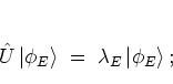 |
(2.18) |
 |
(2.19) |
Since
![]() is an eigenstate of
is an eigenstate of
![]() with respect to the eigenvalue
with respect to the eigenvalue ![]() ,
,
![]() is an eigenstate of
is an eigenstate of
![]() with respect to the
same eigenvalue
with respect to the
same eigenvalue ![]() :
:
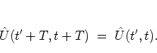
where in the last step the periodicity (2.13) of
![]() has been used.
Therefore
the
has been used.
Therefore
the
![]() can
all
be labelled by the same index
can
all
be labelled by the same index ![]() ,
indicating the same eigenvalue
for all
,
indicating the same eigenvalue
for all ![]() .
.
Because of the unitarity of ![]() its
eigenvalues are of unit modulus and can be written as
its
eigenvalues are of unit modulus and can be written as
The definition (2.23) is tailored to make the description
of the time dependence of the
![]() as similar to the dynamics
of an autonomous system as possible.
What is more, for stroboscopic times these two types of dynamics coincide,
as similar to the dynamics
of an autonomous system as possible.
What is more, for stroboscopic times these two types of dynamics coincide,
Since the parameter ![]() plays a similar role as the energy eigenvalue of a
time-independent system,
plays a similar role as the energy eigenvalue of a
time-independent system,
![]() is
called
a
quasienergy of the time-periodic Hamiltonian, and the
FLOQUET states
is
called
a
quasienergy of the time-periodic Hamiltonian, and the
FLOQUET states
![]() are referred to as its quasienergy states
[Zel67]. For brevity, often the states
are referred to as its quasienergy states
[Zel67]. For brevity, often the states
![]() are
called (reduced) quasienergy states, too.
The
quasienergy is defined modulo
are
called (reduced) quasienergy states, too.
The
quasienergy is defined modulo ![]() only, since
it originates from the exponential in equation
(2.22).
Due to this nonuniqueness of the quasienergy it cannot be identified
with any physical observable
in a straightforward way,
but note that, for an unscaled system, the quasienergy has the dimension
of an energy.
A discussion of the problems potentially arising from identifying the
quasienergy with the conventional energy
-- and thereby linking the quasienergy spectrum directly with the
resonance (emission/absorption) spectrum
of the respective system --
may be found in [DM98].
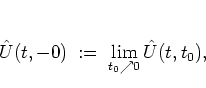
Normally, one restricts
only, since
it originates from the exponential in equation
(2.22).
Due to this nonuniqueness of the quasienergy it cannot be identified
with any physical observable
in a straightforward way,
but note that, for an unscaled system, the quasienergy has the dimension
of an energy.
A discussion of the problems potentially arising from identifying the
quasienergy with the conventional energy
-- and thereby linking the quasienergy spectrum directly with the
resonance (emission/absorption) spectrum
of the respective system --
may be found in [DM98].
Normally, one restricts ![]() to the interval
to the interval
![]() .
By equation (2.21), the case of
.
By equation (2.21), the case of ![]() , i.e.
, i.e. ![]() ,
corresponds to the quantum map's stationary states,
for which not only the reduced
,
corresponds to the quantum map's stationary states,
for which not only the reduced
![]() , but also the full
FLOQUET states
, but also the full
FLOQUET states
![]() are periodic with period
are periodic with period ![]() .
.
The quasienergy states
are characterized by
several useful properties.
It is easy to show that for ![]() the quasienergy states
the quasienergy states
![]() ,
,
![]() are
orthogonal: their scalar product is
are
orthogonal: their scalar product is
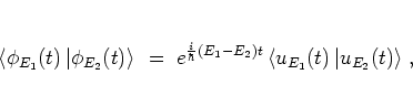 |
(2.26) |
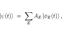
Summarizing, with respect to a time-periodic Hamiltonian the quasienergies and the quasienergy states play much the same role as the energy eigenvalues and the stationary energy eigenstates do with respect to a time-independent Hamiltonian [Sam73]. This analogy includes the observation that in the same way as any solution of the time-independent SCHRÖDINGER equation can be expanded in terms of energy eigenstates with constant coefficients, the same can be accomplished using quasienergy states in the FLOQUET case.