Next: Topological Considerations
Up: Analysis of Real-World Data
Previous: Analysis of Real-World Data
Contents
The first idea one might have about the choice of the sampling time  is to make it as small as possible, such that one can reconstruct a
``smooth'' trajectory in the embedding space. However, this approach is
rather short-sighted [5]: If we choose too small then
consecutive measurements of
is to make it as small as possible, such that one can reconstruct a
``smooth'' trajectory in the embedding space. However, this approach is
rather short-sighted [5]: If we choose too small then
consecutive measurements of  will give nearly the same results,
 |
(18) |
This means that the vectors
 |
(19) |
constructed via the method of delays, will be stretched along the diagonal
in the  -dimensional embedding space and thus the analysis of the
picture of the attractor will be very difficult. To get an intuitive
picture of what is happening in this case one can think of the phase
space picture being artificially compressed towards the diagonal and this
decreases the dimensionality of the attractor although there is no
physical reason for this. In fact, numerical experiments show that for
small sampling times one gets spuriously low results of dimension
calculations, for example the correlation dimension tends to zero as
approaches zero [8].
On the other hand must not be chosen too large, because in this
case the
-dimensional embedding space and thus the analysis of the
picture of the attractor will be very difficult. To get an intuitive
picture of what is happening in this case one can think of the phase
space picture being artificially compressed towards the diagonal and this
decreases the dimensionality of the attractor although there is no
physical reason for this. In fact, numerical experiments show that for
small sampling times one gets spuriously low results of dimension
calculations, for example the correlation dimension tends to zero as
approaches zero [8].
On the other hand must not be chosen too large, because in this
case the  become totally uncorrelated (since one of the features
of a ``chaotic'' system is the exponential separation of nearby
trajectories, and thus the noise which is present in every real system
gives rise to total non-correlation of measurements which are made in
sufficiently large time intervals). This means that the vectors
become totally uncorrelated (since one of the features
of a ``chaotic'' system is the exponential separation of nearby
trajectories, and thus the noise which is present in every real system
gives rise to total non-correlation of measurements which are made in
sufficiently large time intervals). This means that the vectors  fill (the relevant
part of) the embedding space more or less homogeneously and extraction of
any information from this phase space picture becomes impossible
[5].
It is possible to regard this problem of being too large from
another
point of view [8]: We have seen in section 2.2 that one can
also use (instead
of the method of delays) a vector the components of which are the first
derivatives of the observable to construct a phase space picture. Now,
since we cannot measure the derivatives themselves we compute
approximations to them using the time series. It is typical for such
approximation formulae that the error of the approximant is
fill (the relevant
part of) the embedding space more or less homogeneously and extraction of
any information from this phase space picture becomes impossible
[5].
It is possible to regard this problem of being too large from
another
point of view [8]: We have seen in section 2.2 that one can
also use (instead
of the method of delays) a vector the components of which are the first
derivatives of the observable to construct a phase space picture. Now,
since we cannot measure the derivatives themselves we compute
approximations to them using the time series. It is typical for such
approximation formulae that the error of the approximant is
 with some integer
  . (See for example footnote
2 in section
2.2.) This means that to get a sensible result for this
approximation, and thus for , we want to have small!
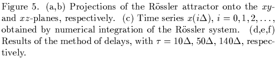
We illustrate the effect of a ``bad'' choice of with a numerical
experiment: We consider a derivate of the Lorenz system, the
Rössler system (see e.g. [14], chapter 5.3), which is
defined by
. (See for example footnote
2 in section
2.2.) This means that to get a sensible result for this
approximation, and thus for , we want to have small!
We illustrate the effect of a ``bad'' choice of with a numerical
experiment: We consider a derivate of the Lorenz system, the
Rössler system (see e.g. [14], chapter 5.3), which is
defined by
For the parameter values  ,
,  ,
,  the flow of this
system becomes attracted to the Rössler attractor, the projections of
which onto the
the flow of this
system becomes attracted to the Rössler attractor, the projections of
which onto the  - and to the
  -planes are shown in Fig. 5.a and
Fig. 5.b, respectively. Numerical integration (with some step size
-planes are shown in Fig. 5.a and
Fig. 5.b, respectively. Numerical integration (with some step size
 ) of eq. (22) provides us, for example, with the time
series
) of eq. (22) provides us, for example, with the time
series
 , depicted in
Fig. 5.c. Using this data and several different delay times , we can
reconstruct (in 2-dimensional embedding space) the phase space pictures
of the Rössler attractor which are shown in Fig. 5.d, ...,
Fig. 5.h9. The effects we described in the above
, depicted in
Fig. 5.c. Using this data and several different delay times , we can
reconstruct (in 2-dimensional embedding space) the phase space pictures
of the Rössler attractor which are shown in Fig. 5.d, ...,
Fig. 5.h9. The effects we described in the above
paragraph for too small
(stretching along the diagonal) and too large (increasing
non-correlation of the data) are clearly visible in Fig. 5.d and Fig. 5.h,
respectively.
So it is clear that a proper choice for the sampling time is a
necessary requirement for the method of delays to give sensible results.
A similar statement holds for the embedding dimension :
Obviously
must be large enough to allow  to be embedded within
  .
The more complex the attractor is the higher must be (see
footnote 7 in section 2.2). What is more, to make sure
that the choice of
allows Takens' theory to be applied one might be tempted to make
very large in order to guarantee that
.
The more complex the attractor is the higher must be (see
footnote 7 in section 2.2). What is more, to make sure
that the choice of
allows Takens' theory to be applied one might be tempted to make
very large in order to guarantee that  .
If is chosen too small then we change the distribution of the points
on the attractor artificially and the point densitiy
.
If is chosen too small then we change the distribution of the points
on the attractor artificially and the point densitiy
 |
(21) |
develops singularities which are absent in an embedding space with
large enough [5]. (As a simple example consider the surface
of a sphere in 3
dimensions which is ``embedded'' in 2 dimensions. Even if the point
density on the sphere in 3-space is constant the ``embedded'' sphere,
which is essentially a projection of the sphere into the plane, will have
singularities on the boundary.) If it is known a priori that the
attractor
is visited uniformly then one can use this observation to determine
the embedding dimension: Take the smallest such that the densitity on
the reconstructed attractor does not have any singularities. However, this
method requires some pre-knowledge about the system and cannot be taken
as a general approach to the choice of .
There are good arguments to
keep small as well: It is easier to work with a low-dimensional
embedding space, especially if one aims at building up some geometrical
intuition about the attractor's shape. Also, working in higher dimensions
results in larger numerical errors when one wants to use the
reconstructed attractor to calculate the usual quantities which
characterize the system, such as the Hausdorff or correlation
dimension [5].
But the best argument not to make too large is perhabs the problem
which we
pointed to in section 2.2: in contrast to Takens' statement that
systems with periods smaller than or equal to  can be excluded
on generic grounds we saw that these periods actually can appear,
generally speaking. So we have to take additional precautions to prevent
such periodic flows with small periods to cause trouble, since otherwise
Takens' theory can not be applied! An easy solution for this problem is to
make
can be excluded
on generic grounds we saw that these periods actually can appear,
generally speaking. So we have to take additional precautions to prevent
such periodic flows with small periods to cause trouble, since otherwise
Takens' theory can not be applied! An easy solution for this problem is to
make  small [7].
Footnotes
- ... 5.h9
-
Fig. 5.d, ..., Fig. 5.h consist of clouds of points, in contrast to
the continuous orbit of the system shown in Fig. 5.a and Fig. 5.b. This is
not an inherent problem of the method of delays, but due to the limited
computing power we had available for this little experiment: By choosing a
smaller step size while keeping constant, we would have
got pictures similar to Fig. 5.d, ..., Fig. 5.h, but consisting of
``quasi-continuous'' orbits.
Next: Topological Considerations
Up: Analysis of Real-World Data
Previous: Analysis of Real-World Data
Contents
Martin_Engel
2000-05-25