Next: Choice of First Embedding
Up: Singular System Analysis
Previous: Choice of a Proper
Contents
We will see that in the presence of noise one has to expect that all zero
eigenvalues  (of the noise-free case) will be changed into
non-zero numbers, small but non-zero! So the simple method of the above
section breaks down and the result of the computation will be in almost
all cases
(of the noise-free case) will be changed into
non-zero numbers, small but non-zero! So the simple method of the above
section breaks down and the result of the computation will be in almost
all cases  , no matter how large
  is.
To deal with this problem we introduce two new matrices
is.
To deal with this problem we introduce two new matrices
The elements of  are called the singular values
of
are called the singular values
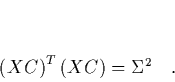
of  . Using these definitions, the definition of
  and eq.
(34) we get the important relation
and eq.
(34) we get the important relation
 |
(38) |
Recall that
 is by definition an orthonormal basis of
 . So the
  -matrix
 can be interpreted
as the projection of the trajectory matrix onto this new basis. Then
can be interpreted
as the projection of the trajectory matrix onto this new basis. Then
 is the trajectory matrix expressed in the basis
  , and
, and
 in the above equation is the covariance matrix in
the same new basis. If one considers the general form of a covariance
matrix,
in the above equation is the covariance matrix in
the same new basis. If one considers the general form of a covariance
matrix,
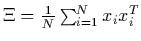 , then it is clear that
measures the correlation of all the vectors
, then it is clear that
measures the correlation of all the vectors  , averaged over
the entire trajectory. Thus the fact that the product
gives a
diagonal matrix (eq. (40)) shows that in the basis
, averaged over
the entire trajectory. Thus the fact that the product
gives a
diagonal matrix (eq. (40)) shows that in the basis  the vectors of the trajectory (
 ) are uncorrelated 13.
What is more, we can see from eq. (40) that
) are uncorrelated 13.
What is more, we can see from eq. (40) that  is
proportional to the extent to which the trajectory varies in the
-direction. One can think of the trajectory as exploring on the
average an ellipsoid in , the directions and lengths of the
axes of which are given by the and the , respectively.
This picture is very valuable for the discussion of the effect of noise
on the trajectory: If there is, for example, a floor of white noise
(i.e. we have
is
proportional to the extent to which the trajectory varies in the
-direction. One can think of the trajectory as exploring on the
average an ellipsoid in , the directions and lengths of the
axes of which are given by the and the , respectively.
This picture is very valuable for the discussion of the effect of noise
on the trajectory: If there is, for example, a floor of white noise
(i.e. we have
 , where
 is the
deterministic contribution to the observable and
is the
deterministic contribution to the observable and  stands for the
noise) then we get for the covariance matrix an expression like
stands for the
noise) then we get for the covariance matrix an expression like
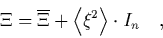 |
(39) |
where
 denotes the time average,
  is the
 -identity matrix and
  is the deterministic
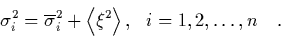
contribution we have discussed until now. Diagonalization of for
this ``white noise case'' yields the eigenvalues
is the deterministic
contribution we have discussed until now. Diagonalization of for
this ``white noise case'' yields the eigenvalues
 |
(40) |
Notice that in the presence of noise all eigenvalues are non-zero
(since
 ), even
for those directions which are not explored by the deterministic
movement of the system. Thus the influence of noise on our analysis is to
make us think that the (deterministic) trajectory explores all
directions of , instead of only
), even
for those directions which are not explored by the deterministic
movement of the system. Thus the influence of noise on our analysis is to
make us think that the (deterministic) trajectory explores all
directions of , instead of only  !
The solution of this problem is found by considering the singular
value decomposition of :
!
The solution of this problem is found by considering the singular
value decomposition of :
 |
(41) |
( is the -matrix formed of the eigenvectors of
  .) We
will see below that this decomposition is useful, because
appears as one of
the factors constituting . We want to find those entries of
which are obviously non-zero only due to the effects of
noise. One possibility to do this is to measure, in addition to the true
time series, a time series which consists only of the noise and then to
compute the corresponding mean square projections onto the
-directions
(which we found for the true time series). These quantities are to
be compared with the respective (of the true time series) and
if both are found to be of
the same order of magnitude then we know that this particular
is only non-zero due to the noise; in other words, the corresponding
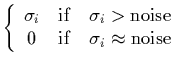
direction is noise-dominated. A straightforward strategy (which
uses the special form of eq. (43)) to get
rid of this most significant
influence of noise is to set those selected entries equal to
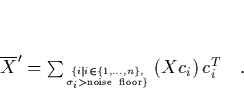
zero14. Thus we arrive at the following corrected equation for the approximate
deterministic part
.) We
will see below that this decomposition is useful, because
appears as one of
the factors constituting . We want to find those entries of
which are obviously non-zero only due to the effects of
noise. One possibility to do this is to measure, in addition to the true
time series, a time series which consists only of the noise and then to
compute the corresponding mean square projections onto the
-directions
(which we found for the true time series). These quantities are to
be compared with the respective (of the true time series) and
if both are found to be of
the same order of magnitude then we know that this particular
is only non-zero due to the noise; in other words, the corresponding
direction is noise-dominated. A straightforward strategy (which
uses the special form of eq. (43)) to get
rid of this most significant
influence of noise is to set those selected entries equal to
zero14. Thus we arrive at the following corrected equation for the approximate
deterministic part  of the trajectory matrix:
(Notice that the
 are not the deterministic
component
are not the deterministic
component
 of the ; but, by construction,
 and
should be approximately the same.),
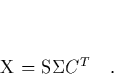
which can be simplified to get a representation of the corrected trajectory
matrix which is most easy to work with:
and
should be approximately the same.),
which can be simplified to get a representation of the corrected trajectory
matrix which is most easy to work with:
 |
(45) |
This equation is nice to work with since the and are easy
to compute by diagonalization of the covariance matrix.
The sum in eq. (47) will run over  summands, and of course we
expect
summands, and of course we
expect  . We relabel the
 such that the
first of them correspond to those eigenvalues which are not
noise-dominated. Then we know, after having eliminated the effect
of noise as far as possible, that the trajectory is confined to a
-dimensional subspace of which is spanned by
such that the
first of them correspond to those eigenvalues which are not
noise-dominated. Then we know, after having eliminated the effect
of noise as far as possible, that the trajectory is confined to a
-dimensional subspace of which is spanned by
 . So we can take
  as the embedding space
instead of .
Finally we get the following vectors on the trajectory in :
as the embedding space
instead of .
Finally we get the following vectors on the trajectory in :
 |
(46) |
and it is these vectors which we can now plot in dimensions (taking
e.g. two- or three-dimensional cross-sections) to get the geometric
picture of the attractor which we have been aiming at.
Footnotes
- ... uncorrelated13
-
This result justifies the choice
 in section 3.1: since in a
well-chosen basis () the vectors which form the trajectory are
uncorrelated, the lag-time does not influence our results and we can
choose it at our convenience.
in section 3.1: since in a
well-chosen basis () the vectors which form the trajectory are
uncorrelated, the lag-time does not influence our results and we can
choose it at our convenience.
- ...
zero14
-
One should be aware of the fact that this strategy does not remove
all effects of the noise on the trajectory: The noise contribution
to those
 which are non-zero according to
eq. (46) remains unchanged. It is not totally
clear to me why Broomhead and King in [7] do not propose to
subtract the noise
floor from all eigenvalues by replacing in
eq. (43) with
which are non-zero according to
eq. (46) remains unchanged. It is not totally
clear to me why Broomhead and King in [7] do not propose to
subtract the noise
floor from all eigenvalues by replacing in
eq. (43) with
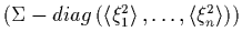 (or with
 in the case of white
noise);
this would (on the average!) remove the noise floor from all eigenvalues.
Maybe the reason for not doing this are:
in the case of white
noise);
this would (on the average!) remove the noise floor from all eigenvalues.
Maybe the reason for not doing this are:
 we would not get eq. (47) in this nice form which
is easy to handle numerically;
we would not get eq. (47) in this nice form which
is easy to handle numerically;
the effect of noise on the first components is assumed to
be not very large;
for the calculation of the numerical values of the
do not matter anyhow, apart from being above or in the
noise floor.
Next: Choice of First Embedding
Up: Singular System Analysis
Previous: Choice of a Proper
Contents
Martin_Engel
2000-05-25