Figure captions

Figure 1.

Magnetic field lines of the magnetic bottle as described by (32) with $B_0=B_2=1$. The full 3-dimensional picture is obtained by rotation about the $z$-axis.

Figure 2.

Typical dynamics in the magnetic bottle at the energy $E=0.5$. The dotted lines show the boundary of the accessible region of the configuration space, defined by the condition $V(\rho,z)\leq E$.

Figure 3.

Poincaré plots of the magnetic bottle at the energy $E$ as described in the text. The boundary of the surface of section, defined by $\vert p_z\vert=\sqrt{2E}$, shows up as horizontal lines. (a) $E=0.01$. (b) $E=0.2$. (c) $E=0.5$.

Figure 4.

The quasi-integral $I^{(m)}(t;{\mbox{\protect\boldmath$s$}})$ of the magnetic bottle (33) plotted as a function of time for several different values of $m$. (a) $E=0.01$, ${\mbox{\protect\boldmath$s$}}=(0,0.05)$. (b) $E=0.2$, ${\mbox{\protect\boldmath$s$}}=(0,0.3)$.

Figure 5.

Convergence plot for the magnetic bottle at the energy $E=0.2$. The same Poincaré surface is shown as in figure 3b. On a $200 \times 200$ grid the convergence function $C({\mbox{\protect\boldmath$s$}})$ has been calculated and the points with $C({\mbox{\protect\boldmath$s$}})=1$ have been marked with black.

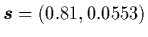
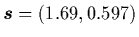
Figure 6.

A typical graph of $\eta^{(m)}({\mbox{\protect\boldmath$s$}})$. A region of pseudo-convergence and a divergent region are separated by $m_0({\mbox{\protect\boldmath$s$}})=8$. The parameters for this picture are $E=0.2$, ${\mbox{\protect\boldmath$s$}}=(0,0.3)$.

Figure 7.

$m_0({\mbox{\protect\boldmath$s$}})$-plots for the magnetic bottle at the same energies as in figure 3. Again the Poincaré surface is shown as a $200 \times 200$ grid of points which are shaded, this time according to their respective values of $m_0({\mbox{\protect\boldmath$s$}})$, as shown in the key. (a) $E=0.01$. (b) $E=0.2$. (c) $E=0.5$.

Figure 8.

Normalized standard deviations $\eta^{(m)}({\mbox{\protect\boldmath$s$}})$ (marked by $\Diamond$) and their approximants $a({\mbox{\protect\boldmath$s$}})e^{\alpha({\mbox{\protect\footnotesize\protect\boldmath$s$}})}$ (solid lines) for the magnetic bottle. The parameters $a({\mbox{\protect\boldmath$s$}})$ and $\alpha({\mbox{\protect\boldmath$s$}})$ have been computed using the data for $m=8,10,12,14$. (a) $E=0.01$; ${\mbox{\protect\boldmath$s$}}=(0.81,0.0553)$. (b) $E=0.2$; ${\mbox{\protect\boldmath$s$}}=(1.69,0.597)$. (c) $E=0.2$; ${\mbox{\protect\boldmath$s$}}=(0,0.3)$.

Figure 9.

$\alpha({\mbox{\protect\boldmath$s$}})$-plot for the magnetic bottle at the energy $E=0.2$. The $200 \times 200$ grid points are shaded according to their respective values of $\alpha({\mbox{\protect\boldmath$s$}})$. The calculation of these values is based on $\eta^{(m)}({\mbox{\protect\boldmath$s$}})$ for $m=8,10,12,14$.