
Consider the well-known Størmer problem which is given by the Hamiltonian
completely describing the classical motion of a charged particle in the earth's magnetic field (which is assumed here to be a pure dipole field).
As the first step of our simplification procedure, we transform from the
ordinary cylindrical polar coordinates
![]() used above to dipolar coordinates
used above to dipolar coordinates ![]() and expand
the resulting expression in terms of these new coordinates and their
corresponding canonically conjugate momenta
and expand
the resulting expression in terms of these new coordinates and their
corresponding canonically conjugate momenta ![]() ,
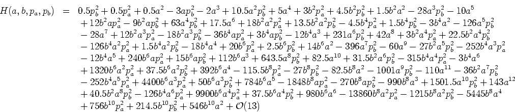
, ![]() (cf. G. Contopoulos, L. Vlahos, J. Math. Phys. 16 (1975) 1469-1474):
(cf. G. Contopoulos, L. Vlahos, J. Math. Phys. 16 (1975) 1469-1474):
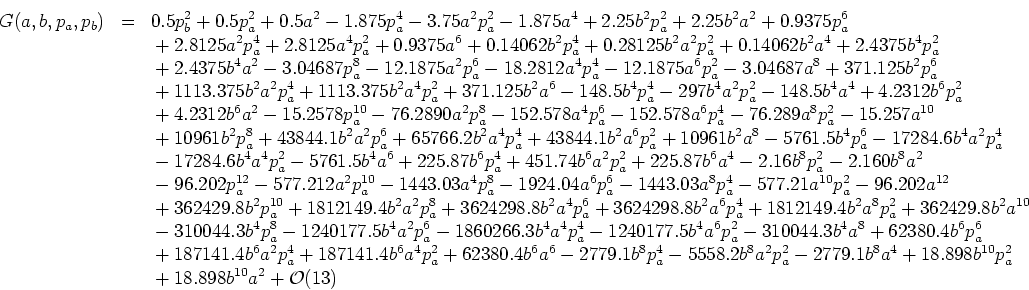
Now generalized normal form theory (U. M. Engel, B. Stegemerten, P. Eckelt, J. Phys. A: Math. Gen. 28 (1995) 1425-1448) can be applied to this transformed Hamiltonian, yielding the following most simple normal form for the Størmer problem:
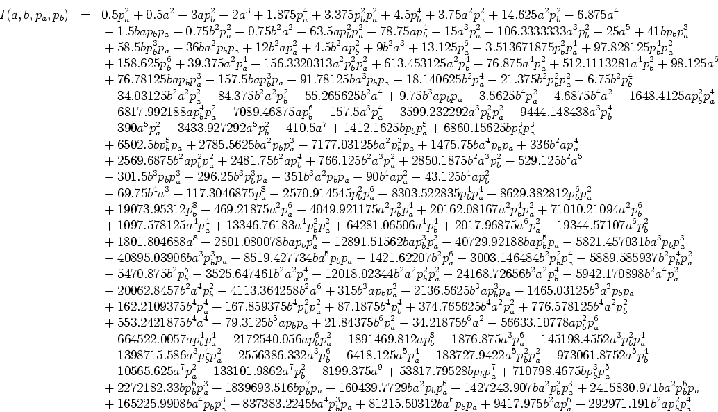
The third, and final, step on our path towards maximum simplicity is the transformation of the above normal form into the corresponding quasiintegral of motion; for our little sample problem, a minute's thought will reveal that we have:
![\begin{eqnarray*}
{}\mbox{{}\rule{2.6cm}{0.0001cm}{}}{} %ME
&&{}
+988776.6406...
...b^3 p_b^5 p_a^3
-109960281.2 b^3 p_b^7 p_a %ME \\ [-0.1cm]&&{}
\end{eqnarray*}](img9.png)
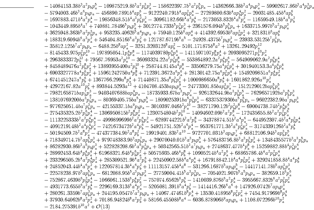
The most impressive simple structure of this tiny little formula and its evident meaningfulness immediately show the superiority of our simplification algorithm.