Appendix: Details of the normalization pro-
cess for a magnetic bottle

In this appendix we discuss some details of the transformation of a Hamiltonian with a quadratic part (34) into generalized normal form. More specifically, we show how to simplify the Lie operator

$${\cal A}_m(\cdot) %% = \left\{ \cdot,H_2(\VEC{z}) \right\} ... ...\partial}{\partial z_{n+\nu}}(\cdot) \right) \right]_{\L _m}$$

which is adjoint to this particular $H_2$.

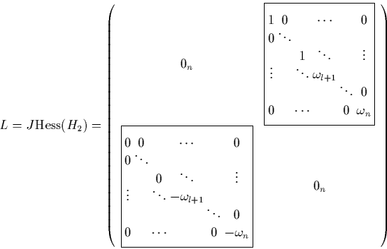
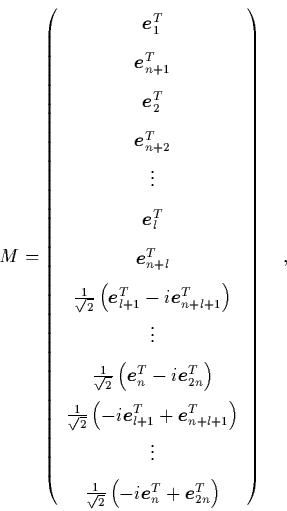
The unitary matrix that by a similarity transformation puts the Hamiltonian matrix

$$L = J \mbox{Hess}(H_2) = \left( \begin{array}{cc} 0_n&\f... ...ts & & 0 & -\omega_n \end{array} $}& 0_n \end{array} \right)$$

into the Jordan normal form $\tilde{L}=MLM^*$ of (35) is

$$M = \left( \begin{array}{c} {\mbox{\protect\boldmath$e$}}_... ...otect\boldmath$e$}}_{2n}^T \right) \end{array} \right) \quad,$$

with ${\mbox{\protect\boldmath$e$}}_i$ being the canonical base vectors of ${\bf R}^{2n}$. This formula can easily be derived by performing a certain permutation of the rows and columns first, followed by a transformation similar to (15).

In the new coordinates $\tilde{{\mbox{\protect\boldmath$z$}}}=M{\mbox{\protect\boldmath$z$}}$ the Lie operator takes on the form

$$\tilde{{\cal A}}_m = \left[ \sum_{\nu=1}^l \tilde{z}_{2\n... ...rtial}{\partial\tilde{z}_{n+\nu}} \right) \right]_{\L _m} \;.$$

This representation of the Lie operator is advantageous, because here we have collected as many non-zero entries (of the matrix representation) of ${\cal A}_m$ on the diagonal as possible. Only the first sum yields an off-diagonal contribution.

We have not yet made any assumptions about the ordering of the monomials $\tilde{{\mbox{\protect\boldmath$z$}}}^{\mbox{\protect\footnotesize\protect\boldmath$j$}}$ in the basis of $\L _m$. If one chooses the lexicographical ordering [2] of the basis monomials, then the matrix representation of $\tilde{{\cal A}}_m$ becomes an upper diagonal matrix for all $m$, and all the manipulations of ${\cal A}_m$ that are necessary in the course of the normalization procedure (solving linear equations, inverting ${\cal A}_m$, ...) become easier and consume much less computing time.

In the case $l=1$ it is possible to achieve even further simplification by an appropriate ordering of the basis monomials of $\L _m$. One can introduce the so-called magnetic bottle ordering of monomials which results in $\tilde{{\cal A}}_m$ being bidiagonal.